Dynamic Programming

Put the lost future back into the model

The previous chapter found a safe rule for unweighted interval scheduling: keep the compatible meeting that finishes first. Now give each meeting a value.

A  [1, 4)   value 5
B  [3, 5)   value 6
C  [0, 6)   value 8
D  [4, 7)   value 5
E  [5, 9)   value 11
F  [8, 9)   value 4

Earliest finish chooses A, D, and F, worth 14. Choosing B and E is worth 17. The greedy exchange still preserves room for later meetings, but it no longer preserves value. A local choice cannot summarize the future.

Brute force can keep both possibilities alive: for each meeting, take it or skip it. That search contains the right choices and the wrong amount of repetition. Many branches eventually ask the same question: what is the best value obtainable from the first i meetings?

Dynamic programming begins when that repeated question is precise enough to answer once.

Name one question that every cell answers

Sort the meetings by finish time. For meeting i, let p(i) be the number of earlier meetings that finish no later than i starts. Define:

best(i) = maximum value obtainable from the first i meetings

The word first refers to finish-time order. It makes best(i) a complete sentence, not a label such as “best so far.” Once the first i meetings are fixed, the path used to reach them cannot affect the remaining choices.

There are only two possibilities for the last meeting among those i:

• Skip it, leaving best(i - 1).
• Take it, earning its value plus best(p(i)) from the compatible prefix.

So the recurrence is:

best(0) = 0
best(i) = max(best(i - 1), value[i] + best(p(i)))

The base case is part of the meaning: with no meetings available, the maximum value is zero. If values could be negative and the prompt required choosing at least one meeting, that base case would describe a different problem and would need to change.

The recurrence is correct because every optimal schedule for the first i meetings either excludes meeting i or includes it. In the first case its value is bounded by best(i - 1). In the second, every other chosen meeting must lie in the compatible prefix ending at p(i), so its value is bounded by value[i] + best(p(i)). The recurrence considers the best schedule in both exhaustive cases.

That proof does more than justify a formula. It establishes that the state has not forgotten anything the future can observe.

Recursion, memoization, and tabulation are execution choices

A direct recursion follows the take-or-skip proof, but it recomputes the same prefixes. Memoization keeps the recursive shape and caches each best(i) the first time it is requested. It is often the cleanest first implementation when only a sparse part of a state space is reachable or the dependency order is awkward to write.

Tabulation evaluates the same recurrence in an explicit dependency order. Here both dependencies, i - 1 and p(i), are smaller than i, so a left-to-right pass is sufficient:

from bisect import bisect_right


def weighted_schedule(intervals):
    """Return (maximum value, one optimal list of interval names)."""
    ordered = sorted(intervals, key=lambda item: (item[2], item[1]))
    ends = [end for _, _, end, _ in ordered]
    best = [0] * (len(ordered) + 1)
    previous = [0] * (len(ordered) + 1)

    for i, (_, start, _, value) in enumerate(ordered, start=1):
        # Search only meetings before i. The result is also the compatible
        # prefix length, which is the index into best.
        previous[i] = bisect_right(ends, start, hi=i - 1)
        take = value + best[previous[i]]
        skip = best[i - 1]
        best[i] = max(skip, take)

    chosen = []
    i = len(ordered)
    while i > 0:
        name, _, _, value = ordered[i - 1]
        take = value + best[previous[i]]
        if take > best[i - 1]:
            chosen.append(name)
            i = previous[i]
        else:
            i -= 1

    chosen.reverse()
    return best[-1], chosen

For the six meetings above, the result is (17, ["B", "E"]). Sorting and the predecessor searches cost O(n log n); the DP and reconstruction passes cost O(n). The array stores n + 1 states.

Notice that reconstruction is not an afterthought. Walking backward compares the choice that produced best(i) with best(i - 1). This implementation skips on ties, deliberately selecting one of possibly several optimal schedules. If the prompt asks for all optimal schedules, a single parent path is no longer enough.

The five agreements in a DP solution

The interval derivation has five parts that must describe the same problem:

1. State: one sentence defining the answer stored for a subproblem.
2. Transition: the exhaustive last choice, move, character, or operation.
3. Base cases: already-known answers with exactly the same meaning.
4. Evaluation order: every dependency is ready before it is read.
5. Answer and witness: the location of the requested value and, when required, a way to recover the choices that produced it.

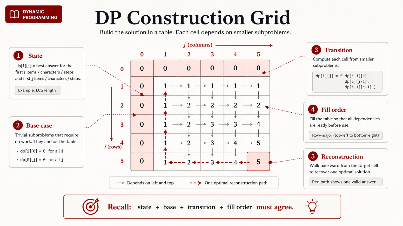
Most DP bugs are disagreements among these parts. A transition may use a prefix state while its base case assumes a suffix. A correct two-dimensional recurrence may be compressed into a loop that overwrites a dependency too early. A score may be correct while the rows needed to reconstruct its witness have disappeared.

The repair is rarely “add another loop.” Say the state sentence again and test every other part against it.

Change the promise, change the state

Problem families are useful only when they suggest a question to investigate. They do not supply a table automatically. The safest way to learn the major families is to change one promise and watch the state respond.

A budget adds a dimension: 0/1 knapsack

In weighted interval scheduling, finish-time order lets compatibility collapse to one prefix index. In 0/1 knapsack, choosing an item changes both which items remain and how much capacity remains. A sufficient state is:

dp[i][c] = maximum value using the first i items with capacity c

For item i - 1, skip from dp[i - 1][c], or take from value[i - 1] + dp[i - 1][c - weight[i - 1]] when it fits. The previous row is essential: each item may be used at most once.

There are nC states and constant work per transition, for O(nC) time. This is pseudo-polynomial, because C is a numeric value rather than the number of bits required to encode it.

Only the previous row is needed for the value, so the table can be compressed to one capacity array. Capacity must then move backward:

for each item:
  for c from capacity down to weight[item]:
    dp[c] = max(dp[c], value[item] + dp[c - weight[item]])

Backward iteration ensures that dp[c - weight[item]] still means “using earlier items.” Moving forward would allow the current item to feed its own row, silently changing 0/1 knapsack into unbounded knapsack. That forward order is correct when reuse is allowed. The same update with a different direction answers a different question.

Subset sum uses the same choice-and-budget geometry with Boolean feasibility instead of maximum value. Coin change may minimize the number of coins or count combinations; one recurrence takes a minimum, while the other adds counts. Similar-looking arrays do not make those meanings interchangeable.

Compression may also destroy reconstruction. If the prompt asks which items were chosen, retain parent decisions, keep the full table, or establish another honest recovery method before discarding rows.

Two prefixes meet: sequence DP

Edit distance asks for the minimum insertions, deletions, and replacements needed to turn one string into another. Its natural state is:

dp[i][j] = minimum operations to turn a[0:i] into b[0:j]

The empty-prefix boundaries follow immediately: dp[i][0] = i deletions and dp[0][j] = j insertions. When the last characters match, the answer is dp[i - 1][j - 1]. Otherwise the last operation is a deletion, insertion, or replacement:

dp[i][j] = 1 + min(
    dp[i - 1][j],
    dp[i][j - 1],
    dp[i - 1][j - 1],
)

The indexes i and j are prefix lengths, so the characters being compared are a[i - 1] and b[j - 1]. Saying that aloud prevents more errors than memorizing the diagram.

Not every sequence state needs two prefixes. For longest increasing subsequence, a useful quadratic state is “the longest increasing subsequence ending exactly at index i.” The answer is the maximum over all ending positions, not necessarily the last cell. The faster binary-search algorithm uses a different invariant; it is not merely this table with less space.

Position becomes relevant: grid DP

On an obstacle-free grid with moves only right and down, the next chapter can count paths directly with a binomial coefficient. Add blocked cells and move order alone no longer determines validity. Position must return to the state:

ways[r][c] = number of valid paths that reach cell (r, c)

A blocked cell has value zero. Any other cell receives the sum from its legal top and left neighbors. The first row is not “initialized to one” by ritual: cells remain reachable only until an obstacle blocks the sole path along that boundary. The state sentence determines the initialization.

If movement includes cycles, a simple fill order may not exist. You may need a larger acyclic state, a graph algorithm, bounded-step DP, or a fixed-point method. Calling the storage a grid does not remove cyclic dependencies.

How small may the state be?

A state is sufficient when histories grouped into the same state have identical legal futures and identical future contribution to the objective. It is minimal when no recorded fact can be removed without breaking that property.

This gives two useful attacks on a proposed state:

• Omission test: find two histories that map to the same state but permit different future choices or values. Their distinguishing fact is missing.
• Redundancy test: remove one variable and ask whether the remaining state still determines every transition and terminal answer.

Stock trading with cooldown, for example, cannot use only the day index. Holding stock, resting, and cooling down permit different next actions. A mode dimension restores that information. Conversely, word break does not need to remember the internal segmentation of a prefix when the prompt asks only whether segmentation is possible. The future needs the end index and the Boolean answer, not the path that produced it.

This is also the boundary with backtracking and greedy reasoning. Backtracking retains distinct paths when the paths themselves must be enumerated or do not merge into reusable state. Greedy erases alternatives only after a proof shows that a local choice or frontier contains everything the future can use. DP keeps several futures, but merges histories once they become equivalent.

Derive before you optimize

In an interview, begin with the choices, not the table dimensions. A compact explanation for the interval problem is:

Taking or skipping a meeting creates an exponential search. After sorting by finish time, many branches ask for the best value from the same compatible prefix. I will store that answer as best(i). The last meeting is either excluded, giving best(i - 1), or included, giving its value plus best(p(i)). Both dependencies are smaller prefixes, so I can fill from left to right and then walk backward to recover one schedule.

That explanation exposes the claims another engineer should challenge: why the state is sufficient, why the cases are exhaustive, why the order is safe, where complexity comes from, and whether the witness can be recovered.

For an unfamiliar prompt, work through the same reasoning:

1. Write the brute-force choices or recursive question.
2. Identify which calls repeat and which history the future can still observe.
3. State the smallest sufficient subproblem in one sentence.
4. Derive exhaustive transitions and meaningful boundaries.
5. Draw the dependency edges; they determine memoization or fill order.
6. Count states and work per transition separately.
7. Locate the final answer and plan reconstruction before compressing space.

Then pressure-test the derivation. Does an omitted transaction count, previous value, capacity, mode, or endpoint change the future? Does loop order reuse an item that should be indivisible? Does a substring operation add cost hidden by the recurrence? Does the answer end anywhere rather than at the last cell? Is a numeric dimension pseudo-polynomial? Each question tests meaning, not visual familiarity.

Practice transfers are strongest when one changed promise invalidates the previous solution. Allow meetings to overlap at a penalty. Require exactly k selected intervals. Change 0/1 knapsack to reusable items. Ask edit distance for an edit script rather than its length. Add diagonal moves or teleporters to a grid. For each variation, say which state, dependency, or reconstruction claim broke before repairing it.

The finished table is evidence of a derivation, never the derivation itself.

Related reading

• Chapter 31: Complexity and Constraint Analysis
• Chapter 46: Recursion, Backtracking, and Divide and Conquer
• Chapter 47: Greedy Algorithms
• Chapter 50: Pattern Selection and Proof