Graphs

When is a state safe to close?

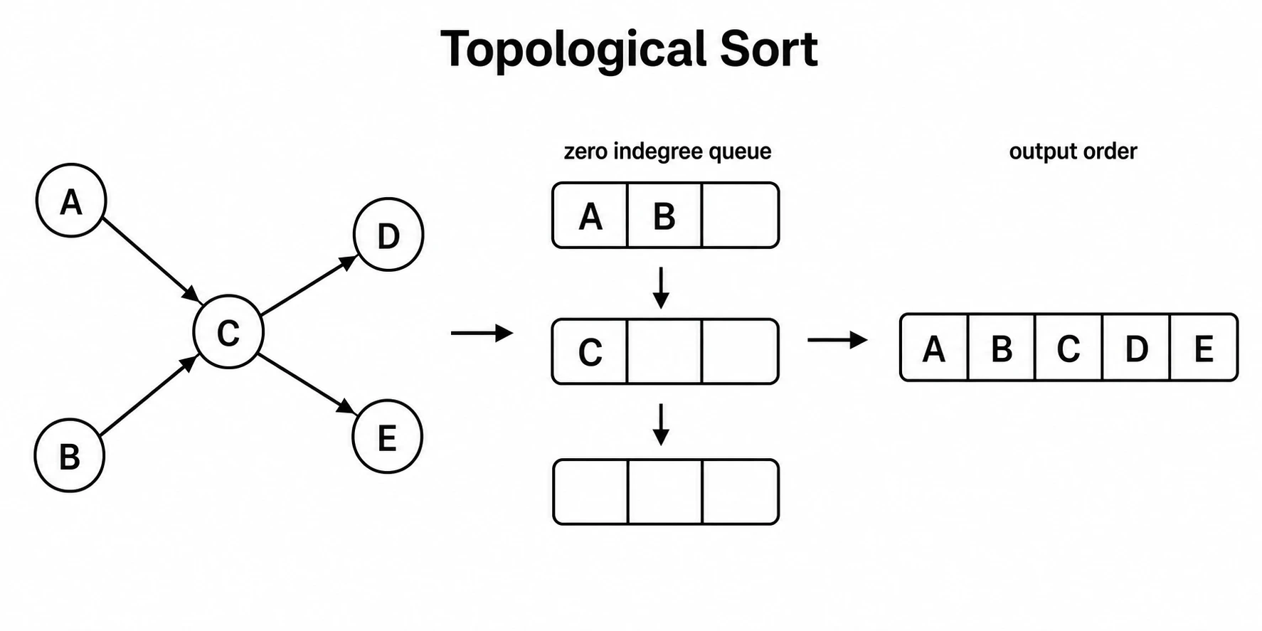
Suppose five services must be deployed. accounts and catalog can start immediately. checkout needs both of them. receipts and search-index each need checkout. A deployment tool must produce a legal order—or explain why no legal order exists.

The service names are vertices. A prerequisite is a directed edge from the service that must finish to the service it unlocks. The problem is not really about deployment, and it is not solved by choosing DFS or BFS from memory. It asks when a vertex has enough evidence to be considered ready.

That question is the center of graph reasoning. A breadth-first search closes a state when its minimum unweighted distance is known. A depth-first search finishes a state after its descendants have been explored. A topological sort emits a vertex when all incoming dependencies have been removed. Dijkstra’s algorithm finalizes a vertex when no cheaper path can arrive later. The data structures differ because the promises differ.

Trees made the previous chapter simpler by promising one rooted, acyclic shape. A graph may lead back to a state already reached, contain several components, or generate neighbors without storing any edges at all. Once those promises disappear, visited state is not optional bookkeeping. It is a claim about which future work can no longer improve the answer.

Build the right graph before searching it

Most failures begin one decision before the algorithm. An edge in the wrong direction can make correct topological-sort code answer the wrong question. A visited key that omits a resource can merge states that have different futures. A representation built only from edge sources can make isolated vertices vanish.

For the deployment example, the edge accounts -> checkout means that accounts must appear first. Reversing every edge would still produce a graph, but its outgoing neighbors and resulting order would mean something else. Name the edge in a sentence before constructing it.

State identity needs the same care. In a plain grid, (row, column) may be a complete vertex. If the traveler may break one wall, then (row, column, break_available) is the state. Reaching a cell after spending the wall break must not prevent another path from reaching the same cell with the resource intact. Word ladders, lock combinations, board positions with a turn indicator, and routes with a limited number of stops all have this property: the visible location may be only part of the vertex.

Choose a representation for the operations the solution performs:

• An adjacency list uses O(V + E) space and is the usual choice when the graph is sparse and traversal needs outgoing neighbors.
• An edge list keeps O(E) input compact and works naturally when processing or sorting edges, as in union-find or Kruskal’s algorithm. Neighbor lookup remains expensive until the edges are indexed.
• An adjacency matrix spends O(V^2) space to make an edge lookup constant time. That exchange can be sensible for a small, dense graph.
• An implicit graph stores no adjacency structure. A grid, puzzle, word transformation, or tuple state generates legal neighbors on demand. The cost of generating those neighbors belongs in the complexity analysis.

If vertices are numbered 0 through n - 1, initialize all n adjacency buckets. If ids are arbitrary, collect vertices from the explicit vertex list and from both ends of every edge. The empty bucket is evidence too: it says the vertex exists and has no outgoing neighbors.

Dependency removal makes ordering inspectable

Return to the deployment graph. Count each vertex’s incoming edges. At the start, only accounts and catalog have indegree zero, so only they can be ready. Removing either one satisfies one prerequisite of checkout; removing both reduces checkout to indegree zero. The process then unlocks receipts and search-index.

from collections import deque


def can_finish(num_courses, prerequisites):
    graph = [[] for _ in range(num_courses)]
    indegree = [0] * num_courses

    for course, prerequisite in prerequisites:
        graph[prerequisite].append(course)
        indegree[course] += 1

    ready = deque(
        course
        for course in range(num_courses)
        if indegree[course] == 0
    )
    completed = 0

    while ready:
        course = ready.popleft()
        completed += 1
        for dependent in graph[course]:
            indegree[dependent] -= 1
            if indegree[dependent] == 0:
                ready.append(dependent)

    return completed == num_courses

The proof is carried by the indegree. Every vertex entering ready has no remaining prerequisite, so appending it after previously removed vertices is safe. Removing the vertex accounts for exactly its outgoing edges. If all vertices are removed, the resulting sequence respects every dependency.

If the queue empties early, the remaining vertices all have positive indegree. Following an incoming edge among a finite set of remaining vertices must eventually revisit one, so a directed cycle exists. This is stronger than saying “the algorithm found fewer vertices”: incomplete processing is the observable consequence of dependencies that can never become ready.

The running time is O(V + E) because each vertex enters the queue at most once and each edge decrements one counter once. The graph, counters, and queue use O(V + E) space. Initializing all vertices is what lets an isolated course participate in that proof.

Depth-first search provides a different view of the same cycle. Give each vertex one of three states: unseen, active, or finished. A DFS marks a vertex active on entry and finished only after every outgoing neighbor is finished. An edge to an active vertex returns to the current dependency chain and proves a cycle. An edge to a finished vertex is harmless; that work was completed on another branch. A single visited set cannot preserve this distinction.

DFS postorder, reversed, gives a topological order when no active-edge cycle is found. Kahn’s algorithm is often preferable when readiness is the natural story or when a partial schedule is useful. DFS colors are often preferable when the recursive dependency path itself is useful for diagnosing a cycle.

Frontier order determines the guarantee

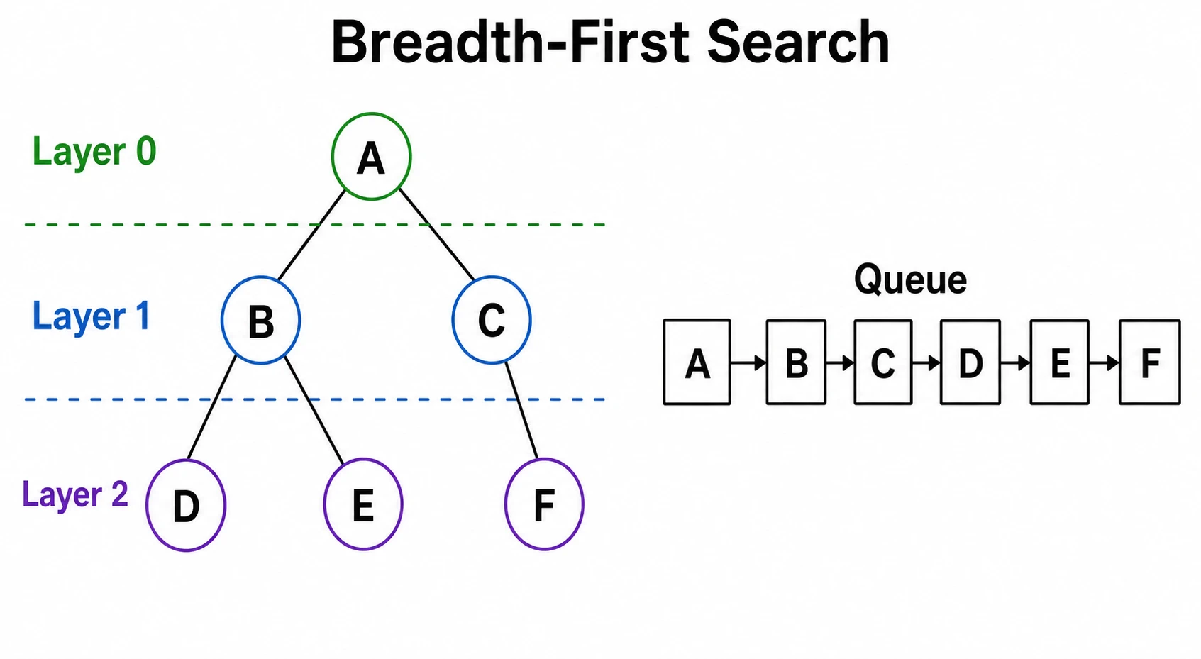
Now change the question. Instead of asking for a legal order, ask for the fewest dependency hops from one service to another in an unweighted graph. Every edge costs one, so the frontier must advance by distance layer.

from collections import deque


def unweighted_distances(start, neighbors):
    distance = {start: 0}
    queue = deque([start])

    while queue:
        node = queue.popleft()
        for neighbor in neighbors(node):
            if neighbor not in distance:
                distance[neighbor] = distance[node] + 1
                queue.append(neighbor)

    return distance

Here distance is also the visited set. The invariant is that every queued vertex already has its minimum edge distance. When a vertex at distance d discovers an unseen neighbor, every vertex at a smaller distance has already been processed or is ahead in the queue. No path with fewer than d + 1 edges can arrive later.

Mark on enqueue, not dequeue. If two vertices in one layer both point to the same neighbor, dequeue-time marking schedules that neighbor twice and can overwrite its parent. Enqueue-time marking makes first discovery authoritative because the FIFO order has already proved its distance.

Multi-source BFS is the same proof with several distance-zero states. Put all initial sources in the queue and distance map before the loop. Rotting fruit, nearest facilities, and distance to any exit often take this form.

DFS changes the frontier from a FIFO queue to a call stack or explicit stack. It remains excellent for reachability, component marking, and exhaustive exploration, but first discovery no longer implies minimum distance. Mark a vertex before exploring its neighbors so a cycle cannot schedule the same work indefinitely. Prefer an explicit stack when graph depth can exceed the language’s call-stack limit.

On an implicit grid with four-direction movement, V = rows * columns and each cell generates at most four edges, so E = O(V). A word ladder may have far more expensive neighbor generation; saying O(V + E) is correct only if the construction or generation cost represented by E has actually been counted.

Components change with the meaning of connection

To count islands, scan every cell. When an unseen land cell appears, it begins one component; a BFS or DFS then claims every land cell reachable from it. The outer scan matters because a traversal from one start cannot discover another component.

The grid can serve as its own visited set by changing claimed land to water, but only when mutation is permitted. Otherwise keep a separate set. With fixed-direction neighbors, the scan and traversal take O(RC) time. A recursive DFS can also consume O(RC) stack frames when one island fills the grid, so an iterative frontier may be the safer implementation even though the asymptotic work is unchanged.

“Connected” is incomplete language for a directed graph. It may mean reachable from one start, weakly connected after ignoring directions, or strongly connected, where every vertex in the component can reach every other vertex. Clarify which relation defines the component before counting it.

When undirected edges arrive over time and the recurring question is whether two vertices are now connected, repeated traversal throws away useful work. Disjoint-set union, or union-find, stores a representative for each component:

class DisjointSet:
    def __init__(self, size):
        self.parent = list(range(size))
        self.rank = [0] * size

    def find(self, node):
        if self.parent[node] != node:
            self.parent[node] = self.find(self.parent[node])
        return self.parent[node]

    def union(self, left, right):
        left_root = self.find(left)
        right_root = self.find(right)
        if left_root == right_root:
            return False

        if self.rank[left_root] < self.rank[right_root]:
            left_root, right_root = right_root, left_root
        self.parent[right_root] = left_root
        if self.rank[left_root] == self.rank[right_root]:
            self.rank[left_root] += 1
        return True

Path compression shortens future find operations; union by rank avoids building a tall parent tree. Across a sequence of operations, their amortized cost is effectively constant for ordinary input sizes (O(α(V))). A failed union says the new undirected edge joins vertices already in one component, which is exactly the redundant-edge or undirected-cycle signal many prompts need.

Union-find deliberately forgets route shape. It cannot reconstruct a path, respect directed reachability, produce a dependency order, or find a shortest route. Use it when component membership is the answer, not merely because the input contains edges.

Coloring asks whether every edge can cross a partition

A bipartite graph can assign one of two colors to every vertex so adjacent vertices always receive different colors. Start any uncolored component with color zero. BFS or DFS then gives every unseen neighbor the opposite color; an edge whose endpoints already share a color proves failure.

The component loop is essential. One component may be a valid chain while a disconnected component contains an odd cycle. Team assignment, mutual-dislike constraints, and “split into two compatible groups” prompts often hide this shape, but the edge meaning must really be an undirected opposite-group constraint. Two-coloring does not solve arbitrary scheduling or directed dependency rules.

The invariant is local and global at once: every processed edge crosses the partition, and every colored vertex has a color consistent with the path that reached it. Encountering the same vertex through a path of incompatible parity reveals an odd cycle.

Weighted edges require a stronger notion of finality

A FIFO queue proves minimum edge count, not minimum cost. If one edge costs ten and two edges cost one each, the one-edge route may be discovered first and still be worse. For nonnegative weights, Dijkstra’s algorithm orders the frontier by the cheapest tentative distance:

from heapq import heappop, heappush


def shortest_paths(start, graph):
    distance = {start: 0}
    frontier = [(0, start)]

    while frontier:
        cost, node = heappop(frontier)
        if cost != distance[node]:
            continue

        for neighbor, weight in graph.get(node, []):
            next_cost = cost + weight
            if next_cost < distance.get(neighbor, float("inf")):
                distance[neighbor] = next_cost
                heappush(frontier, (next_cost, neighbor))

    return distance

A vertex may enter the heap several times as cheaper routes are found. The stale-entry check discards a pair whose cost is no longer current. With nonnegative weights, when the current cheapest pair is popped, any alternate route to that vertex must first pass through a frontier state of equal or greater cost and then add a nonnegative edge. It cannot improve the popped distance. That is the finalization proof.

Negative edges break it: a route processed later can reduce the cost of a vertex already treated as final. Bellman–Ford-style relaxation handles negative edges and can detect reachable negative cycles, at a higher cost. When weights are only zero or one, a deque gives a sharper special case: place a zero-cost move at the front and a one-cost move at the back. For a small dense graph requiring all-pairs distances, Floyd–Warshall’s O(V^3) dynamic program may be simpler than running many single-source searches.

The useful selection rule is therefore precise:

• Use BFS when every move has equal cost and minimum steps matter.
• Use 0–1 BFS when weights are exactly zero or one.
• Use Dijkstra when weights are nonnegative and may differ.
• Use an algorithm that permits repeated relaxation when negative weights are possible; also decide what a reachable negative cycle means for the answer.

Change one promise at a time

Practice graph reasoning by forcing the invariant to change, not by collecting unrelated templates.

Begin with reachability between two vertices. Then require the minimum number of unweighted edges and explain why the stack must become a queue. Add several equally near starting vertices and initialize a multi-source frontier. Give the edges nonnegative costs and explain why discovery is no longer final and the queue must become a min-heap.

Build a course scheduler next. Return a legal order, then introduce a cycle and return one diagnostic dependency chain. Kahn’s processed count answers the first request cleanly; DFS active-state colors make the second request easier. The graph did not change, but the evidence required from the traversal did.

Count components in an undirected edge list, including isolated vertices. Then accept edges one at a time and answer repeated connectivity queries. The static traversal should give way to union-find. Ask for the actual path between two vertices, and union-find is no longer sufficient.

Finally, search a grid in which one wall may be removed. Trace two arrivals at the same cell—one with the removal still available, one without it. If the visited key merges them, construct the smallest case that loses the only valid route. This exercise exposes state identity more effectively than another memorized traversal.

Five questions before the first edge is explored

Before writing a graph solution, answer:

1. What is the complete identity of a vertex, including resources or history that can change its future moves?
2. What does an edge mean, which direction does it point, and what does it cost?
3. Which guarantee is required: reachability, minimum steps, minimum cost, dependency order, component membership, or a valid two-coloring?
4. What orders the frontier, and at what moment is a state discovered, active, finished, emitted, or finalized?
5. Does the complexity include every vertex, edge, generated neighbor, heap entry, and path or output the solution must produce?

Those answers make the algorithm inspectable. They also reveal when two similar-looking prompts are different problems. Graph fluency is not knowing that BFS uses a queue. It is knowing what the queue proves—and noticing the moment the model no longer permits that proof.

Related reading

• Chapter 31: Complexity and Constraint Analysis
• Chapter 33: Correctness Before Cleverness
• Chapter 44: Trees and Tries
• Chapter 46: Recursion, Backtracking, and Divide and Conquer