Trees and Tries

What must cross this edge?

Consider a function that must decide whether a binary tree is height-balanced: at every node, the heights of the two child subtrees may differ by at most one. The root cannot answer by inspecting its children. It needs facts that exist only after those children have inspected their own descendants.

That is the useful way to see a tree. Each edge is an information boundary. A parent may send context down it; a child may return a summary up it; a breadth-first traversal may use it to construct the next frontier. Correctness depends less on remembering “DFS” than on naming the information that crosses the edge.

This discipline works because a rooted tree makes a powerful promise. Every child belongs to one parent, and the descendants reached through different child edges do not overlap. A call can move to a strict child, solve a smaller instance, and return without needing a visited set. If the input may contain a cycle or a shared child, that proof has already failed; the next chapter’s graph discipline is required.

Let the answer choose the traversal

Suppose the balance check begins at a node whose left and right subtrees have not yet been measured. The parent must wait. This is postorder: descendants are processed before their parent.

def is_balanced(root):
    def height_or_failure(node):
        if node is None:
            return 0

        left_height = height_or_failure(node.left)
        if left_height == -1:
            return -1

        right_height = height_or_failure(node.right)
        if right_height == -1:
            return -1

        if abs(left_height - right_height) > 1:
            return -1
        return max(left_height, right_height) + 1

    return height_or_failure(root) != -1

The helper’s contract is exact: it returns the subtree’s height if that subtree is balanced, and -1 otherwise. An empty subtree returns height zero. A parent combines two successful heights, or propagates failure without doing more work.

That single return value carries two facts because the sentinel cannot be a legitimate height. A tuple such as (is_balanced, height) would be equally valid and may be preferable when sentinel values are easy to confuse. What matters is that the parent receives everything it needs. Returning only a Boolean would leave it unable to compare heights; recomputing height separately at every node can turn a linear traversal into quadratic work on a long chain.

The proof follows the code. The empty tree is balanced and has height zero. Assume each child call correctly reports either its height or a failure. If either child failed, the current subtree also fails. Otherwise the current subtree is balanced precisely when the two heights differ by at most one, and its height is one plus the larger child height. Every call moves to a strict child, so each reachable node is processed once.

This is O(n) time. Its auxiliary space is O(h), where h is the height of the tree—not automatically O(log n). A balanced tree has logarithmic height; a tree that has collapsed into a chain has linear height and may overflow a language’s call stack.

Other traversal orders follow from different contracts:

• When a child needs ancestor context—depth, a path sum, inherited permission, or the valid range for a search-tree node—visit the node before descending. This is preorder.
• When a parent needs a child summary—height, size, balance, diameter, or a candidate ancestor—collect child results first. This is postorder.
• Inorder visits the left subtree, node, and right subtree. It produces sorted values only because a binary search tree adds an ordering invariant; inorder has no universal “sorted” meaning for an arbitrary binary tree.
• When the answer is organized by distance from the root, use a queue. Level order exposes minimum depth, per-level aggregates, and breadth-first views. Its space is O(w), where w is the maximum width.

Preorder, inorder, and postorder describe when a node is handled relative to its children. DFS and BFS describe how the frontier is managed. Keeping those ideas separate makes it easier to derive a traversal instead of reaching for a name.

Recursion is an implicit data structure

The recursive balance solution stores unfinished work in call frames. An iterative version must store the same work explicitly; changing syntax does not remove the state.

For a preorder traversal, a stack of nodes is enough:

def preorder(root):
    if root is None:
        return []

    result = []
    stack = [root]
    while stack:
        node = stack.pop()
        result.append(node.val)
        if node.right is not None:
            stack.append(node.right)
        if node.left is not None:
            stack.append(node.left)
    return result

The right child is pushed first because the stack reverses processing order. Postorder needs more information: a frame must distinguish “I have just arrived” from “my children are complete.” One common representation is (node, expanded). On the first visit, push the node back as expanded and then schedule its children; on the expanded visit, combine their facts.

Prefer recursion when the subtree contract is clear and the maximum depth is safe. Prefer an explicit stack when depth is untrusted, when the language has a small recursion limit, or when pausing and resuming traversal requires precise control. Prefer a queue when the required guarantee is about levels or minimum edge distance. These are operational decisions, not tests of elegance.

Information can travel down as well as up

A binary search tree is valid only if every node respects all of its ancestors, not merely its parent. The following tree passes local parent-child checks and is still invalid:

    10
   /  \
  5    15
      /  \
     6    20

The 6 is below 15 on a left edge, but it remains in the right subtree of 10; therefore it must be greater than 10. The missing information is an ancestor range carried downward.

def is_valid_bst(root):
    def valid(node, low, high):
        if node is None:
            return True
        if not (low < node.val < high):
            return False
        return (
            valid(node.left, low, node.val)
            and valid(node.right, node.val, high)
        )

    return valid(root, float("-inf"), float("inf"))

Here the arguments mean that every value in this subtree must lie strictly between low and high. The code assumes values compare safely with those sentinels and duplicates are forbidden. If duplicates are legal, “BST” is not a complete specification: the insertion and lookup contract must say which side receives equality, and validation must use the same rule.

This distinction also prevents a common complexity claim from slipping past inspection. Search, insertion, predecessor, and successor in an ordinary BST cost O(h). They are O(log n) only when some balancing invariant keeps the height logarithmic. AVL trees, red-black trees, and other balanced search trees pay rotation and metadata costs to preserve that guarantee under updates. A heap is shape-balanced but does not provide arbitrary ordered lookup. A sorted array gives cheap search and expensive middle insertion. A hash table gives expected constant-time exact lookup but no predecessor, successor, or range order. The operation the caller needs—not the word “tree”—chooses among them.

Lowest common ancestor needs an identity contract

For two nodes in a general binary tree, the lowest common ancestor is the lowest node whose subtree contains both targets. That definition makes the information flow postorder: each subtree must report which targets it found.

A familiar compact implementation returns a node when it encounters either target and merges two nonempty child results at their meeting point. It is correct only when both targets are known to exist. If one is missing, it may return the other target as though it were a complete answer.

When existence is part of the problem, preserve it in the returned fact:

def lca_if_both_exist(root, p, q):
    """Assume p and q are distinct node objects."""

    def search(node):
        if node is None:
            return None, 0

        left_answer, left_count = search(node.left)
        right_answer, right_count = search(node.right)

        count = left_count + right_count
        if node is p or node is q:
            count += 1

        if left_answer is not None:
            return left_answer, count
        if right_answer is not None:
            return right_answer, count
        if count == 2:
            return node, count
        return None, count

    answer, found = search(root)
    return answer if found == 2 else None

Node identity is deliberate. If values may repeat, comparing node.val can find the wrong objects. If p and q may be the same node, decide whether that single object counts as both targets and handle that contract separately.

In a BST, ordering can replace the subtree search. If both target values are lower than the current value, move left; if both are higher, move right; otherwise the paths split at the current node. That faster movement is earned by the BST invariant and by assumptions about target existence and duplicate placement. It is not a generic LCA trick.

Serialization must preserve absence

Values do not determine a binary tree’s shape. A root 1 with a left child 2 and a root 1 with a right child 2 produce the same two values under preorder unless missing children are represented.

  1        1
 /          \
2            2

Preorder with null markers gives each possible child slot an answer:

def serialize(root):
    tokens = []

    def visit(node):
        if node is None:
            tokens.append("#")
            return
        tokens.append(str(node.val))
        visit(node.left)
        visit(node.right)

    visit(root)
    return ",".join(tokens)

Deserialization consumes the same contract in the same order:

def deserialize(data, Node):
    tokens = iter(data.split(","))

    def build():
        token = next(tokens)
        if token == "#":
            return None
        node = Node(int(token))
        node.left = build()
        node.right = build()
        return node

    root = build()
    try:
        next(tokens)
    except StopIteration:
        return root
    raise ValueError("trailing tokens")

Each value token claims exactly two following subtree encodings; each # closes one child slot. A production format also needs framing, escaping or a typed encoding, malformed-input behavior, and perhaps a version. Level-order encoding can work too, but it needs an equally precise convention for nulls and omitted trailing slots. Parent-pointer trees, n-ary trees, and graphs have different shape information and therefore need different formats.

A trie turns the path into evidence

A trie changes what an edge means. Instead of “this is a child in the hierarchy,” an edge consumes the next token of a key. Reaching a node after the letters t, e, a proves that some stored key has that prefix. It does not prove that tea itself was stored.

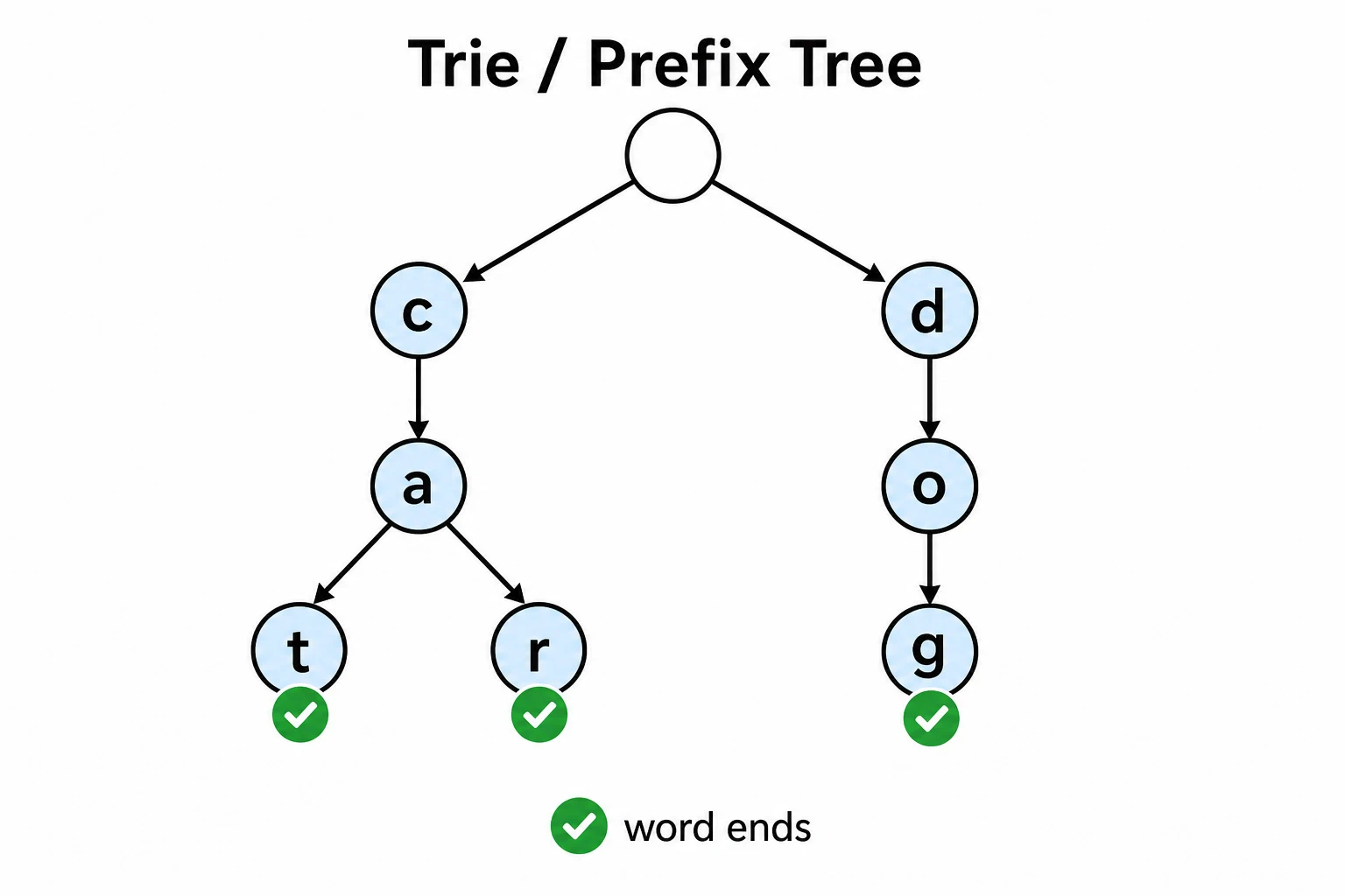
That final fact requires a terminal marker:

class TrieNode:
    def __init__(self):
        self.children = {}
        self.terminal = False


class Trie:
    def __init__(self):
        self.root = TrieNode()

    def insert(self, key):
        node = self.root
        for token in key:
            if token not in node.children:
                node.children[token] = TrieNode()
            node = node.children[token]
        node.terminal = True

    def _walk(self, text):
        node = self.root
        for token in text:
            node = node.children.get(token)
            if node is None:
                return None
        return node

    def search(self, key):
        node = self._walk(key)
        return node is not None and node.terminal

    def starts_with(self, prefix):
        return self._walk(prefix) is not None

With hash-map children, these operations take expected O(L) time for a key of length L, apart from output work. The representation determines the real cost. A fixed child array gives direct indexing for a small known alphabet but wastes slots in sparse nodes. A radix tree compresses single-child paths at the price of more complicated splits. For a static dictionary, a sorted array and two binary searches may be smaller and simpler than a pointer-heavy trie.

Autocomplete exposes the output contract. Walking to a prefix node is only O(L); finding the best suggestions below it costs additional traversal. A mostly static, read-heavy service can cache a small ranked list at each node, making queries predictable while increasing memory and update work. A system with frequent renames may prefer to traverse on demand or maintain a separate search index. “Use a trie” begins the design; it does not finish it.

Tries also work over path segments, bytes, or words. The tokenization rule must match lookup. Unicode normalization, case folding, locale-sensitive ordering, and ranking are product semantics, not details a character trie solves by itself.

A hierarchy is not a tree until you prove it

Practical hierarchy data often arrives as rows rather than nodes:

id  parent_id  name
1   null       Engineering
2   1          Platform
3   1          Product
4   2          Runtime

It is tempting to build a children_by_parent map and recurse from the row whose parent is null. That traversal can silently omit orphans and disconnected cycles. Before relying on tree algorithms, establish the promised shape.

First require unique ids and decide whether the input describes one rooted tree or a forest. Every non-root parent id must resolve. No child may acquire two parents. Then prove acyclicity and reachability: a color-marking traversal can reject a node reached while active, and the final visited count can expose rows not reachable from the declared roots. If sibling order affects output, define and apply it explicitly rather than inheriting database or hash-map order.

The data carried down the validated tree also needs a contract. Permission hierarchies may inherit, override, or deny; configuration trees may merge maps while replacing lists; filesystem names may be unique only among siblings. “Walk the hierarchy” is incomplete until precedence and identity are stated.

This is the boundary between trees and graphs. A shared child may be a valid directed acyclic graph rather than bad data. Multiple roots may be a valid forest. A cycle may be meaningful in a network. Once those shapes are allowed, do not conceal them behind a tree traversal: model vertices, edges, visited state, and components directly.

Change the contract, not just the input

To practice tree reasoning, make each variation force a different fact across an edge.

Start with maximum depth, whose empty subtree returns zero and whose parent needs only one number from each child. Then compute diameter. The parent still returns its height upward, but the complete answer must also retain the best path found anywhere below. Decide whether to return both facts or keep one carefully scoped accumulator, and explain why no path is lost.

Implement lowest common ancestor once under the promise that both distinct node objects exist. Then remove that promise. The interesting change is not a new test case; it is the richer returned fact that distinguishes a candidate from evidence that both targets were found.

Serialize a binary tree with null markers and round-trip empty, one-sided, and duplicate-valued trees. Then impose a requirement to reject truncated and trailing input. The traversal order can stay the same while the format contract becomes honest.

Build a trie with insert, exact search, and prefix search. Add deletion only after deciding whether nodes shared by another key may be removed. Add top-three autocomplete only after choosing the ranking rule and the update workload.

Finally, build the row-based hierarchy above, then introduce an orphan, a duplicate id, a second root, and a two-node cycle. For each case, decide whether the right result is rejection, a forest, or a graph. The durable skill is not recursion. It is knowing which structural promise permits the recursion to be simple.

The fact at every boundary

Before writing a tree or trie solution, ask four questions:

1. What does an edge mean in this structure?
2. What context must the parent send down, and what fact must the child return?
3. What does an empty child contribute?
4. Which promise prevents revisiting a node?

Those answers determine traversal order, state, proof, and space cost. They also reveal when the input has stopped being a tree. At that moment, adding a visited set is not a patch to the same solution; it is evidence that the problem has crossed into graph reasoning.

Related reading

• Chapter 31: Complexity and Constraint Analysis
• Chapter 33: Correctness Before Cleverness
• Chapter 43: Sorting, Searching, and Intervals
• Chapter 45: Graphs