Capacity Planning, Load Testing, and Cost Modeling

The Replay Fits. The Launch Fits. Together, They Do Not.

Consider a modeled capacity review for the same commerce system. The team has corrected three weeks of revenue history. The replacement job can finish overnight while ordinary traffic continues, and a new customer analytics view has passed its launch test. Both statements are true. They are also dangerously incomplete.

The analytics view will open first to the three largest merchants. Its historical queries begin with cold caches. Search indexing and the nightly close still run in the background. The revenue replay reads old partitions, writes shadow output, and drives an independent reconciliation scan. Tested separately, each workload stays inside the service objective. When they overlap, storage I/O saturates, replica lag grows, and p99 latency fails long before aggregate CPU looks alarming.

Capacity planning exists for this collision. It is a hypothesis about how a particular workload becomes resource use, which limit appears first, how the system behaves near that limit, and how much time an operator needs to act. The hypothesis must be specific enough to lose an argument with a load test.

“We can add nodes” cannot lose such an argument. A useful claim can:

At launch load, cold historical reads plus the correction replay will exhaust primary I/O before CPU because each replayed event updates indexed shadow output and each cache miss competes for the same storage path. Rising disk queue depth and replica lag should precede the p99 breach. If the replay is capped at 20 percent of measured I/O headroom and the three launch tenants are warmed in sequence, live traffic should remain inside its latency objective.

That paragraph names the workload, the predicted constraint, the evidence, and the proposed control. The load test now has something worth disproving.

Count Work, Not Requests

Requests per second describe the outside of a system. Capacity is consumed by the work those requests create. One order can write the order, update inventory and payment state, append an outbox row, maintain several indexes, invalidate a cache, replicate a log record, and later feed search and analytical paths. One dashboard view can perform permission checks, read aggregates, fetch recent events, scan a historical range, and fan out across tenants or partitions.

The commerce team therefore begins with measured production work, not a round QPS target. It separates point reads from scans, writes from retries, interactive traffic from exports, and foreground work from compaction, backup, reconciliation, indexing, retention deletion, and replay. It records ordinary and peak rates, the peak-to-average ratio, concurrency, connection count, cache hit rate, largest-tenant size, hot-key distribution, partition count, retained bytes, and daily growth.

Then it writes four operating states in prose. The current state says what happens during an ordinary peak, including background work. The target state adds the analytics rollout and expected growth. The stress state overlaps plausible pressures: three large tenants, a retry burst, and the nightly close. The recovery state asks the system to keep serving while it replays, restores, reindexes, fails over, or refills caches. Recovery is not spare-time work. Shadow output, reconciliation, and rollback retention all need real capacity while the old answer is still serving.

Data shape matters as much as request rate. Eighteen months of retained events produce a different working set, index height, compaction burden, backup volume, and replay time from one week of synthetic fixtures. A single large merchant can create a hot partition even when total traffic remains modest. Write amplification grows with indexes, replicas, logs, materialized views, and downstream events; read amplification grows with fan-out, cache misses, joins, permission checks, and poorly bounded scans. The plan must follow those multipliers until it reaches the resources that can saturate.

Name the First Constraint

The first constraint is rarely “the database” in the abstract. It is a resource or coordination boundary with observable behavior.

CPU may be spent parsing queries, serializing results, encrypting traffic, compressing data, merging files, evaluating expressions, or multiplying one API call into many storage calls. Memory pressure may evict the useful working set, spill sorts to disk, inflate connection overhead, or lengthen garbage-collection pauses. Primary data is only part of storage: indexes, replicas, logs, snapshots, temporary files, object versions, tombstones, archives, and restore environments all occupy space and change the rate at which it fills.

I/O can bind writes, analytical scans, compaction, backups, reindexing, cold reads, and recovery even while CPU appears comfortable. Network can bind cross-region replication, large result sets, object movement, or partition rebalancing. Connections, locks, partition heat, metadata operations, file counts, and coordination work can fail before a familiar host metric reaches its threshold. Distributed capacity is often limited by the busiest shard or slowest dependency, not the fleet average.

The team predicts primary I/O first because the launch and repair share that path. It expects cold reads to evict useful pages while the replay reads old partitions and writes indexed candidates. Replica lag is a consequence, not a separate mystery: the replica must consume the additional write stream while also serving launch reads. CPU, memory, network, connections, partition heat, and storage growth remain in the observation set so the test can reveal that the prediction was wrong.

This is the useful humility in capacity work. A wrong prediction caught in a representative test improves the model. A vague prediction can survive every test without teaching anything.

Make the Test Uncomfortable on Purpose

The first test had warm caches, uniformly distributed tenants, short histories, no correction replay, and no nightly close. It measured a system that production would never operate. The revised test preserves the shape that can change the result.

Representative data includes historical depth, tenant skew, deleted records, realistic row and object sizes, index cardinality, file and partition counts, and the largest plausible tenant. Sensitive values can be masked or synthesized; the engine-relevant shape cannot be polished away. Representative concurrency includes connection bursts, overlapping transactions, long-lived queries, consumer rebalances, and retries after a downstream timeout. The same requests per second can behave very differently when they arrive through more concurrent work.

The test starts with empty application and storage caches, then opens the historical view for the largest merchant. Two more large merchants follow rather than being averaged into a uniform key distribution. A few long-tail operations—an audit search, a customer export, a deep historical scan, and a support query—arrive at production-like intervals. Search indexing and the nightly close remain active. Finally, the correction replay begins at its proposed rate, writes shadow output, and runs reconciliation against the authoritative totals.

The run does not stop when the traffic generator stops. The team watches whether queues drain, replicas catch up, compaction settles, caches recover, and delayed work finishes inside its deadline. A system can survive a burst and remain impaired for the next hour.

Evidence follows the hypothesis. The report includes p95 and p99 latency, error and retry rates, disk queue depth, read and write throughput, cache hit rate, replication and consumer lag, partition heat, connections, locks, CPU, memory, network, storage growth, hourly cost, and recovery time. A maximum can expose a stall that a percentile hides, but it needs the surrounding trace to distinguish one measurement glitch from a real pause.

The revised test breaks the original plan. At the uncapped replay rate, disk queue depth rises first. Replica lag follows, then p99 historical reads cross the objective. CPU never exceeds the team’s warning threshold. Pausing the replay restores live latency; resuming it at a lower rate keeps both the serving path and the overnight correction deadline healthy. Warming one launch tenant at a time removes the sharpest cache-fill spike. The evidence has not proved unlimited capacity. It has found an operable envelope for this event.

Headroom Buys Time to Intervene

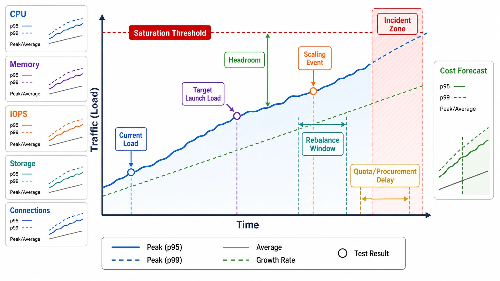
Unused capacity is not automatically headroom. Headroom is reserved capacity for a named failure, burst, recovery action, or scaling delay. Its size depends on the criticality of the workload, the time needed to detect pressure, the time needed to make a decision, and the time needed for new capacity to become useful.

The commerce team can throttle its replay within minutes, but adding storage capacity and rebalancing data takes hours. A quota increase could take longer. Its scaling trigger must therefore fire before the forecast enters that lead-time window. “Scale at 80 percent” says nothing about whether 80 percent is safe. A smooth workload with minute-scale expansion may tolerate a smaller reserve than a bursty workload that needs an eight-hour rebalance. The threshold should be tied to observed behavior: p99 latency, queue depth, replica lag, restore time, partition heat, or another signal that reveals the actual constraint.

Autoscaling does not cancel this reasoning. A platform may scale compute while leaving partitions, storage throughput, connection pools, metadata capacity, downstream services, quotas, or licenses unchanged. It may also add instances faster than data can rebalance into them. The useful question is not whether an autoscaler exists, but which constrained resource it changes and how long that change takes under load.

The plan names a trigger, action, owner, and lead time together. If forecasted I/O crosses the tested operating envelope inside the rebalance window, the data-platform owner starts the scale action. If p99 and replica lag rise together during the replay, the replay controller reduces its rate automatically and the operator decides whether to pause it. If one tenant approaches the tested safe share of a partition, that tenant moves before the next large onboarding. If retained bytes make restore time threaten the recovery objective, the team changes the storage or retention plan before free space becomes the emergency.

Cost the Margin and the Recovery

Capacity and cost are the same model viewed from different sides. The workload assumptions that consume resources also create spend. The model should show ranges and sensitivities rather than a precise-looking total built on guesses.

Storage cost includes retained facts, indexes, replicas, logs, snapshots, archives, temporary files, delayed deletion, and the restore environment. Compute includes steady serving, peak reserve, background jobs, migration windows, replay, and failover capacity. Request charges and egress may appear in object reads, search indexing, stream processing, cross-region replication, partner exports, warehouse scans, and observability. Backups cost more than stored bytes when restore tests, temporary capacity, and operator time are counted.

The team calculates an expected case for ordinary launch traffic and a stress case for cold cache, large tenants, retries, and replay overlap. It varies retention, cache hit rate, write amplification, read amplification, and replay deadline one at a time to see which assumption moves the result. If a small drop in cache hit rate doubles read cost or breaks p99, cache behavior is a capacity dependency. If meeting a four-hour correction deadline requires an expensive emergency cluster while an eight-hour deadline fits existing reserve, the business can decide what the faster repair is worth.

Developer and on-call time belong in that decision. A low infrastructure price can be offset by manual partition repair, fragile scaling, rare expertise, constant tuning, or recovery tooling the team must build and rehearse. Conversely, buying permanent reserve for a rare bounded job may be wasteful when the job can be throttled safely. The model should expose the trade, not smuggle a preferred answer into the spreadsheet.

Leave an Operable Capacity Record

A useful capacity record is short enough to revisit and specific enough to stop a launch. After the test, the commerce team’s record reads:

Decision and deadline:
  Launch historical analytics to the three largest merchants while revenue v2
  is rebuilt overnight. Live p99 and the correction deadline must both hold.

Measured workload:
  Record ordinary and peak reads and writes, 12:1 peak-to-average ratio,
  18 months of retained events, tenant and partition skew, connection count,
  cache hit rate, nightly close, indexing, and reconciliation load.

Capacity hypothesis:
  Primary I/O saturates before CPU when cold historical reads overlap replay
  writes. Disk queue depth and replica lag should rise before p99 fails.

Falsifying test and result:
  Use production-shaped history, empty caches, skewed tenant traffic, long-tail
  queries, active indexing and close, and a rate-controlled replay. Uncapped
  replay breached p99; the tested cap and staged warming kept both workloads
  inside their objectives and allowed the system to catch up afterward.

Headroom and controls:
  Reserve measured I/O for live traffic and failover. Throttle replay on p99,
  disk queue depth, or replica-lag thresholds. Warm one launch tenant at a time.
  The data-platform on-call may pause replay or launch.

Scaling trigger and lead time:
  Start the storage scale action when forecast demand enters the measured
  rebalance window; confirm quota before launch. Split or move a tenant when it
  reaches the tested safe share of a partition.

Cost range and sensitivities:
  Include storage, indexes, replicas, backups, replay compute, requests, egress,
  observability, and operator time. Recalculate for lower cache hit rate, longer
  retention, a larger tenant, and a shorter correction deadline.

Revisit:
  Review after launch, after the correction, and monthly while workload shape is
  changing. Add any incident-discovered pressure to the next load test.

The numbers and thresholds belong in the real record; this example shows the reasoning they must support. A monthly or quarterly review may be enough for a stable system. A launch, large customer, retention change, migration, recovery exercise, or incident demands an immediate revision. Forecast error is evidence. It should change the bottleneck prediction, the test, the trigger, or the cost range.

Change One Variable, Then Combine Them

Choose one production data path and double request rate, retained data, and largest-tenant size separately. For each change, predict the first constraint and design the smallest test that could disprove you. Then combine two pressures that can plausibly meet: cold cache and failover, replay and live traffic, backfill and backup, or a large import and compaction. Name the signal that stops the work, the time needed to add usable capacity, and the cost of keeping or acquiring that margin.

Production traffic should revise a capacity model, not create the first one. Schema and index migrations introduce locks, rewrites, backfills, log volume, and temporary storage. They are safer when the system already knows what work consumes its margin and who can stop before that margin disappears.