Performance Engineering and System Design Handbook / Chapter 55
Analytical Models and Queueing Networks
Build compact calibrated models that rank performance alternatives, expose dominant stations, and reveal their own missing mechanisms through residuals.
Preparing audio…
Audio edition
Analytical Models and Queueing Networks
Use this chapter when a design review has several plausible optimizations, experiments are expensive, telemetry exposes resource demand but not the best change, capacity must be bounded before procurement, or a previously useful model has started disagreeing with the system.
Canopy Analytics has a modeled mean response time of 95.18 ms at 40 correct interactive queries/s. The design target is below 60 ms before the team spends a week building and testing one of three proposals:
| Proposal | Change to the model | Predicted mean | Model verdict |
|---|---|---|---|
| halve API CPU service per visit | 4 ms → 2 ms | 92.59 ms | cannot meet the target; reject as the primary change |
| exact prefilter reduces database visits | 1.6 → 1.2 visits/query | 46.39 ms | can meet the modeled target; test correctness and demand stability |
| route evenly across two database partitions | one → two effective partitions | 43.59 ms | can meet the modeled target; test balance, migration, and failure capacity |
The API optimization is real: it removes two milliseconds of service and slightly more residence time once queueing is included. It is also aimed at the wrong term. The database station contributes 19.2 ms of service demand per completion, runs at modeled utilization 0.768, and contributes 82.76 ms of mean residence. Halving a four-millisecond API term cannot remove 35 milliseconds from the end-to-end mean.
The model does not authorize the prefilter or partition migration. It narrows the next experiment. The prefilter is the cheaper candidate if it can preserve exact query results and the new visit ratio under representative skew. The partition design predicts another 2.79 ms improvement, but it introduces state placement, balance, region-loss capacity, and migration work. A controlled benchmark and Chapter 54’s failure-capacity plan still decide. The model has already paid for itself by removing the attractive local optimization from the critical path.
An analytical model is a deliberately incomplete executable argument. Its value is not realism by volume. Its value is to connect a declared boundary, workload, assumptions, measured coefficients, and decision so transparently that a wrong prediction teaches the team what mechanism is missing.
Write the decision on the model before the equations
A model should begin with six fields:
- Decision: which alternatives, limit, or next measurement will it choose?
- Boundary: where does work enter and where does a correct completion leave?
- Population: which operations, outcomes, tenants, paths, and system states are included?
- Outputs: mean response, utilization, throughput ceiling, cost, or another quantity the model is capable of predicting.
- Calibration evidence: which telemetry or benchmark observations determine its parameters?
- Retirement conditions: what change or residual makes the model unfit for the decision?
Canopy’s boundary is one correct interactive query from gateway admission through API work, result-cache lookup, database visits, and an optional object fetch. The calibration interval is an eight-minute steady population with 40 correct completions/s and a declared operation mix. The decision is which proposal can reduce modeled mean response below 60 ms before controlled testing. The model does not predict p95 or p99, transient overload, retries, priority scheduling, correlated station service, or region failure.
That exclusion is part of the result. A mean queueing model cannot satisfy a tail SLO merely because its output has milliseconds. It can identify a dominant mean-demand station and compare structural alternatives; Chapter 52’s load experiment and Chapter 53’s uncertainty method must test the actual distribution.
Service demand turns telemetry into conserved work
For resource or station i, define:
X: correct system throughput, completions/s;V_i: average visits to stationiper completion, visits/completion;S_i: mean service time per visit, station-s/visit;D_i = V_i S_i: service demand, station-s/completion;U_i: station utilization, a fraction over the same interval.
For a flow-balanced interval with a single normalized unit of station capacity, the utilization law is:
U_i = X × D_i
The units expose mistakes:
(completions / s) × (station-s / completion) = station
The dimensionless station fraction is meaningful only after capacity normalization is declared. For a group of m equivalent parallel servers, aggregate busy time per completion is still D_i, while average utilization per server is approximately X × D_i / m under balanced routing. Do not divide by a server count that jobs cannot actually use because of pinning, partition ownership, licenses, or concurrency gates.
Canopy’s baseline ledger is simulated:
| Station | Visits/completion | Service/visit | Demand/completion | Utilization at 40/s | M/M/1 mean residence |
|---|---|---|---|---|---|
| API | 1.00 | 4.0 ms | 4.0 ms | 0.160 | 4.76 ms |
| result cache | 1.00 | 2.0 ms | 2.0 ms | 0.080 | 2.17 ms |
| database | 1.60 | 12.0 ms | 19.2 ms | 0.768 | 82.76 ms |
| object fetch | 0.25 | 18.0 ms | 4.5 ms | 0.180 | 5.49 ms |
| network total | — | — | 29.7 ms | — | 95.18 ms |
Service demand can be calibrated from busy time divided by correct completions. At the database, the mix has 32 interactive queries/s at 16 ms of database demand and 8 exports/s at 32 ms:
B_db = 32/s × 0.016 s + 8/s × 0.032 s = 0.768 busy-s/s
D_db = (0.768 busy-s/s) / (40 completions/s)
     = 0.0192 busy-s/completion
The arithmetic is operational; the interpretation is conditional. Busy time must cover the same population and include all visits attributable to a correct completion. If dropped work consumes database time, dividing only by successes can legitimately reveal amplification, but the label must say so. If background compaction is excluded from station busy time while competing for the same device, the demand underestimates capacity consumption. If operation mix changes, one average demand is no longer stable.
Keep class coefficients when classes differ:
U_i = Σ_c X_c D_(c,i)
This is the bridge from Chapter 54’s workload forecast to a queueing model. Forecast each class, retain state-dependent demand ranges, and recompute station utilization instead of scaling one blended request count forever.
A queueing network is a map of waiting opportunities
The simplest useful network names stations, visit ratios, service demands, capacity, and routing. It need not reproduce every process. It must include every station that can dominate the decision.
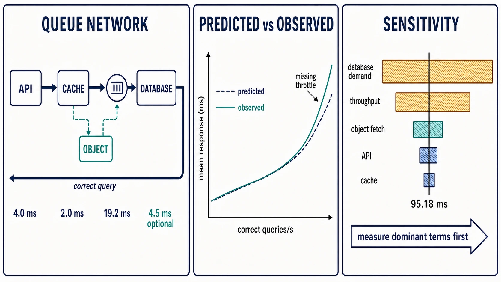
For a teaching station with Poisson arrivals, exponential service, one server, first-come first-served scheduling, an infinite queue, no abandonment, and utilization below one, the M/M/1 mean residence per visit is:
R_(visit,i) = S_i / (1 − U_i)
With V_i average visits and D_i = V_i × S_i, its per-completion contribution is:
R_i = D_i / (1 − X × D_i)
The Canopy total is the sum of station contributions because the model treats them as serial demand on the completion path:
R = Σ_i R_i = 95.18 ms
This is not a generic formula for arbitrary networks. A bounded worker pool rejects or blocks rather than admitting an infinite stationary queue. Priority changes which class waits. Batch arrivals and variable query plans violate memoryless assumptions. A database may have many devices, locks, and schedulers rather than one equivalent server. Use the M/M/1 calculation as a transparent nonlinear comparison only while its assumptions remain tolerable for the decision.
Appendix C supplies M/M/m, Kingman-style variability, queue-age, bottleneck, interactive, and drain cards. Chapter 55’s additional discipline is composition: connect models only when their populations, units, and state agree.
Serial time sums; parallel completion takes an order statistic
For one request with measured serial spans, elapsed critical-path time is the sum of non-overlapping serial work and wait. The sum should be computed per request; adding component p99 values invents a request whose components may never have been slow together.
For parallel branches, completion time depends on the join rule:
- wait for all: the parallel block completes at the maximum branch time;
- wait for any: it completes at the minimum eligible branch time, subject to cancellation and correctness;
- wait for a quorum: it completes at the relevant ordered completion;
- optional branch with deadline: it may leave abandoned work after the caller proceeds.
If branch completion variables are T_1, …, T_n, an all-branch join is:
T_join = max(T_1, …, T_n)
Therefore the mean of the maximum is not the maximum of branch means. Averages discard the information needed to compose parallel tails. Use traces or distributions, preserve dependence, and include cancellation and continued work.
Suppose Canopy fans an exact query to eight shards and every shard must respond. If shard completion times are independent and identically distributed with CDF F(t), then:
P(T_join ≤ t) = F(t)^8
If one shard has a 0.99 probability of completing by 50 ms, the request probability of at least one shard missing 50 ms is:
1 − 0.99^8 = 0.0773
About 7.73% of requests exceed that shard threshold in this narrow model, even though each shard misses it only 1% of the time. Reducing fan-out from eight to four gives:
1 − 0.99^4 = 0.0394
That improvement is not a free recommendation. Fewer shards may increase each shard’s data and service demand. Independence is often false: shared network paths, garbage collection, host throttling, cache state, and request complexity correlate branches. Positive correlation can change the maximum distribution substantially. Measure joint traces or resample complete request vectors; never fabricate a request tail by randomly pairing unrelated shard samples.
Closed populations push back on arrival rate
An open system receives arrivals from outside according to a schedule that need not slow when the service slows. A closed interactive system has a fixed population that alternates between thinking and waiting for the system. Response time feeds back into throughput.
For N users, mean think time Z, system throughput X, and mean response R, the interactive response-time law is:
N = X × (R + Z)
With 120 analysts, 2.0 seconds of mean think time, and observed 0.48-second mean response:
X = 120 / (2.0 + 0.48) = 48.39 queries/s
If the system slows, the same 120 users generate fewer new queries because more users are already waiting. A closed benchmark can therefore make overload look self-healing. An open production event may continue at the offered rate and grow a queue. Match the generator model to user behavior and test both when uncertainty matters.
Two asymptotic bounds catch impossible closed-system predictions. With no queueing, throughput cannot exceed roughly N / (Z + D_sum), where D_sum is the sum of no-wait service demands on the request path. Independently, no saturated station can exceed its service-demand ceiling. For Canopy’s database:
X_(max,db) = 1 / D_db = 1 / (0.0192 s/query) = 52.08 queries/s
The 48.39/s interactive observation sits below that modeled ceiling. As population grows, throughput approaches the bottleneck ceiling while response grows. This bound is not safe goodput: failure headroom, imbalance, background work, SLO limits, and demand variability lower the operational boundary.
Bottleneck laws rank capacity before queue details
For a single-capacity station, the largest demand D_i has the smallest throughput ceiling 1 / D_i. With m_i equivalent usable servers, a first ceiling is m_i / D_i. This comparison requires no exponential distribution and is often the most durable result in the model.
Canopy’s no-wait demands are 4.0 ms, 2.0 ms, 19.2 ms, and 4.5 ms. The database is the baseline bottleneck. Halving API demand raises the API ceiling from 250/s to 500/s, but the database ceiling remains 52.08/s. The local CPU result improves while the system constraint does not move.
The prefilter changes the database demand to:
D′_db = 1.2 visits/query × 12 ms/visit = 14.4 ms/query
At 40/s, modeled database utilization falls from 0.768 to 0.576, and M/M/1 residence falls from 82.76 ms to 33.96 ms. That nonlinear wait reduction is why the whole model reaches 46.39 ms.
Two balanced partitions keep 19.2 ms of total service demand per query but split arrivals evenly. Each partition’s modeled utilization is 40 × 0.0192 / 2 = 0.384. The query still consumes its full database service; the per-query database residence becomes approximately:
R′_db = 0.0192 / (1 − 0.384) = 31.17 ms
This alternative is invalid if one hot tenant remains on one partition, a query fans out to both partitions, or state cannot be partitioned without coordination. “Two databases” is not m = 2 unless routing and ownership make both units usable for the population being modeled.
Scalability curves summarize contention and coherency
Linear scaling assumes each added worker contributes the same useful capacity without adding shared waiting or coordination. A compact empirical alternative is the rational scalability form:
C(N) = N / [1 + α(N − 1) + βN(N − 1)]
where C(N) is capacity relative to one worker, N is concurrency or replicas in the fitted experiment, α is a contention-like term, and β is a coherency or pairwise-coordination-like term. With α = 0.035 and β = 0.0012, the teaching curve is:
| N | relative modeled capacity |
|---|---|
| 1 | 1.000 |
| 8 | 6.097 |
| 16 | 8.825 |
| 32 | 9.770 |
| 48 | 8.968 |
The curve predicts a plateau and then retrograde capacity. It does not prove that “contention” and “coherency” are two observed components merely because the coefficients have names. Several mechanisms—locks, cache invalidation, load imbalance, barriers, allocator contention, shared I/O, or coordination messages—can create the same shape. Fit only within the measured workload and concurrency range, preserve uncertainty, inspect residuals, and use profiles or traces to identify mechanisms.
A fitted scalability curve is especially dangerous after an architecture change. Partitioning may reduce shared-state coordination and change both coefficients; batching may increase useful work per synchronization; a new skew distribution may invalidate the fit. Recalibrate rather than carrying coefficients as platform constants.
Sensitivity tells the team what must be measured well
A point prediction hides coefficient uncertainty. Sensitivity analysis varies one assumption or a coherent scenario and recomputes the decision. At 40 queries/s, varying selected Canopy inputs by ±15% produces:
| Input varied | low-case mean | change | high-case mean | change |
|---|---|---|---|---|
| database demand | 59.43 ms | −35.75 ms | 201.47 ms | +106.28 ms |
| throughput | 67.39 ms | −27.79 ms | 177.16 ms | +81.98 ms |
| object-fetch demand | 94.21 ms | −0.97 ms | 96.22 ms | +1.04 ms |
| API demand | 94.36 ms | −0.83 ms | 96.06 ms | +0.88 ms |
| cache demand | 94.83 ms | −0.35 ms | 95.54 ms | +0.36 ms |
This is the chapter’s sensitivity tornado in text form. Database demand and throughput dominate because their product sits near the nonlinear boundary. The result directs measurement effort: narrow uncertainty in database visits, class mix, and service demand before spending time estimating cache microseconds.
One-at-a-time variation can miss dependence. A launch may raise throughput, export share, database visits, and cache misses together. Add scenario sensitivity that preserves those relationships. Use ranges justified by measurement or forecast evidence; arbitrary ±10% bars create visual symmetry, not uncertainty.
Decision robustness matters more than precise output. The API proposal remains above 60 ms over plausible coefficient ranges, so rejecting it as the primary change is robust. The prefilter sits well below 60 ms in the point model, but a changed result mix or loss of exactness can invalidate the proposal for correctness reasons before performance uncertainty matters.
Calibration is a repeated comparison, not a one-time fit
Calibrate coefficients from aligned telemetry or controlled benchmarks:
- define the completion population and interval;
- measure class throughput and station busy time at several loads below collapse;
- compute visit ratios and service demand with units;
- verify flow balance, correct completions, queue/admission behavior, and generator headroom;
- predict quantities not directly used to fit each point;
- plot observed minus predicted values against load, class, tenant, time, and system state;
- investigate structured residuals before adding coefficients.
Canopy’s baseline model predicts this response curve:
| Correct throughput | predicted mean | observed mean | residual / predicted |
|---|---|---|---|
| 10/s | 34.68 ms | 35.2 ms | +1.5% |
| 20/s | 42.55 ms | 43.9 ms | +3.2% |
| 30/s | 57.16 ms | 58.8 ms | +2.9% |
| 35/s | 70.68 ms | 73.1 ms | +3.4% |
| 40/s | 95.18 ms | 105.0 ms | +10.3% |
| 44/s | 136.37 ms | 178.0 ms | +30.5% |
Random measurement noise would scatter around zero without an obvious shape. These residuals rise with load and bend sharply at the last point. That pattern says the model is missing a load-dependent mechanism or its service demand is no longer constant.
The investigation aligns container CPU bandwidth and finds throttling beginning near 40/s and severe at 44/s. The baseline network has no quota station, so it underpredicts wall time. The wrong response is to refit database service demand upward until the curve matches. That would blame the database for guest scheduling delay and corrupt lower-load predictions. Add an explicit quota mechanism or limit the model’s calibration range, then test again. Chapter 15 supplied the cross-layer clue; the residual made it relevant to this model.
Residuals can expose other omissions:
| Residual pattern | Possible missing mechanism | Decisive next evidence |
|---|---|---|
| error grows with one tenant, not fleet throughput | skew, partition hot spot, class-demand mixture | tenant/shard throughput, demand, queue age, visit ratio |
| sawtooth over time | garbage collection, credits, periodic compaction, autoscaling | aligned runtime/controller/background-work timeline |
| underprediction only on cache miss | mixed service distribution hidden in one mean | hit/miss class demand and routing |
| correct mean, wrong tail | dependence, variability, fan-out, priority, retry | per-request traces and distribution-preserving model |
| overprediction after batching | demand coefficient changed with batch size | service demand and useful work per batch |
| failure-state error | capacity, routing, or recovery work differs | scenario-specific topology and demand ledger |
Do not celebrate a high coefficient of determination while residuals remain structured. A model can track the dominant trend and still be wrong exactly at the decision boundary.
Keep an assumption register beside the result
| Assumption | Evidence or calibration | Failure signal | Action |
|---|---|---|---|
| interval is approximately stationary and flow-balanced | arrivals, correct completions, and backlog change reconcile | growing backlog or changing mix | use a transient model or split intervals |
| demand is per correct useful completion | busy-time ledger reconciles by class | retries, drops, or background work grow | add work classes and amplification |
| baseline station approximation is M/M/1 | low-load curve and service variability are tolerable for ranking | priority, bounds, high variability, blocking | use direct queue age, G/G/1 sensitivity, M/M/m, simulation, or experiment |
| visits and demand stay stable inside an alternative | trace/benchmark coefficients remain in range | plan, cache, payload, or state change | recalibrate alternative coefficients |
| shard completions are independent for fan-out identity | joint traces show weak dependence in scope | shared-event clusters | preserve joint vectors or model correlation |
| two partitions receive balanced usable work | key/tenant distribution and ownership support split | hot partition or cross-partition fan-out | model each partition and coordination |
| scalability coefficients transfer | same build, workload, topology, and range | residual or mechanism change | refit or retire |
An assumption register is not a legal disclaimer. Each row must change measurement or action. If an assumption cannot be tested and the decision is sensitive to it, the model cannot support that decision.
Retire or quarantine the model when operation mix leaves its calibration range, service demand drifts materially, routing or admission changes, retries or throttling become a new station, failure state becomes the decision, or the output required is a tail or transient quantity the model cannot represent. Canopy’s fixture also triggers review when absolute residual exceeds 15% at two adjacent points; direct evidence of a newly active throttle is sufficient sooner.
Communicate a model as a decision packet
A useful review packet is short enough to challenge:
- the exact decision and rejected alternatives;
- boundary, population, state, and success outcome;
- topology with stations, routes, visits, and parallelism;
- parameter table with units, evidence type, date/version, and uncertainty;
- equations with validity conditions;
- observed-versus-predicted curve and residuals;
- sensitivity ranking and scenario ranges;
- correctness, overload, failure, and recovery exclusions;
- next experiment, stop rule, and model retirement owner;
- machine-readable fixture and reproduction command.
Never present extra decimal places as confidence. Canopy’s fixture computes 95.182243… ms so arithmetic checks can be exact; the manuscript reports 95.18 ms because the coefficients do not justify microsecond precision. Label outputs modeled, inputs measured or simulated, and decisions conditional.
Field exercise: reconstruct the model
Using the chapter ledger:
- recompute every station demand and utilization at 40/s;
- derive the 95.18 ms baseline under the M/M/1 teaching assumptions;
- rank the three alternatives by modeled response;
- explain why the API change cannot meet 60 ms;
- name two correctness or transfer risks for the prefilter and two for partitioning;
- use the response residuals to choose the next measurement;
- state which claim cannot be made about p99.
Then change the mix to 24 interactive queries/s and 16 exports/s while keeping each class’s database demand. Aggregate database busy demand becomes 24 × 0.016 + 16 × 0.032 = 0.896 busy-s/s. At the same 40 completions/s, blended database demand becomes 22.4 ms/query and modeled utilization becomes 0.896. Recompute response and decide whether one blended model is still a responsible artifact. The arithmetic should make the mix risk impossible to hide.
Principal drill: decide when analysis must become simulation
Canopy now has eight shards, two priority classes, a bounded admission queue, deadline cancellation, one retry for a declared transient error, cache warming after failover, and a quota that throttles bursty proxy CPU. Interactive users are a closed population, while scheduled exports are open-loop. The team asks for p99 during region loss and recovery.
Produce two artifacts:
- the smallest analytical model that still gives useful demand, bottleneck, fan-out, and population bounds;
- a list of interactions that invalidate its response prediction and must move to Chapter 56’s discrete-event simulation or a controlled resilience test.
A strong answer keeps operational laws for resource accounting and ceilings, preserves class-specific demand, and refuses to derive p99 from station means. It sends priorities, bounded admission, retry feedback, cancellation races, correlated fan-out, failover cache state, quota periods, and recovery scheduling into simulation or experiment. It also defines calibration traces and a test that can falsify the simulator.
Evidence and transfer limits
- Denning and Buzen, “Operational Analysis of Queueing Networks” develops measurable operational quantities, flow balance, visit ratios, bottleneck analysis, and interactive-system relationships. These laws do not make every stochastic queue formula assumption-free.
- Gunther, “A General Theory of Computational Scalability Based on Rational Functions” derives the rational scalability form used for the contention/coherency teaching curve. A fitted coefficient is not an observed mechanism without supporting evidence.
- NIST, “Analysis of Residuals” provides the general model-checking discipline behind inspecting residual structure rather than relying on an aggregate fit statistic.
- Appendix C is the handbook’s point-of-use reference for Little’s Law, M/M/1, M/M/m, Kingman-style approximation, bottleneck and interactive laws, queue age, and backlog drain, with the assumptions attached.
- All Canopy values and observed points are simulated teaching evidence reproduced by
examples/performance-engineering-system-design-handbook/part-06/analytical-queue-network/. The fixture proves arithmetic identities and structural checks only.
The decision rule is: use the smallest calibrated model that can distinguish the alternatives, expose its assumptions and sensitivity, and treat structured residuals as evidence of missing mechanisms. Retire the model when the system or decision crosses its boundary.
Some systems remain analytically useful only at the bounds. Once routing, retries, deadlines, distributions, failures, and policies interact, the next honest move is not a larger spreadsheet. It is a reproducible simulation or trace-replay experiment whose behavior is calibrated back to observed reality.