Performance Engineering and System Design Handbook / Chapter 54
Capacity Planning and Demand Forecasting
Translate operation mix, service demand, uncertainty, failure policy, and lead time into safe capacity, redesign triggers, and marginal economics.
Preparing audio…
Audio edition
Capacity Planning and Demand Forecasting
Use this chapter when a launch, seasonal peak, retention change, regional expansion, hardware order, quota request, or architectural ceiling must become a dated capacity decision rather than a line that says “traffic is growing.”
Canopy Analytics appears comfortable. Its three regions contain 288 query cores, while the current peak mix consumes an estimated 48.22 core-equivalents. A CPU-only chart does not cross installed capacity during the twelve-month plan. That is the wrong chart and the wrong conclusion.
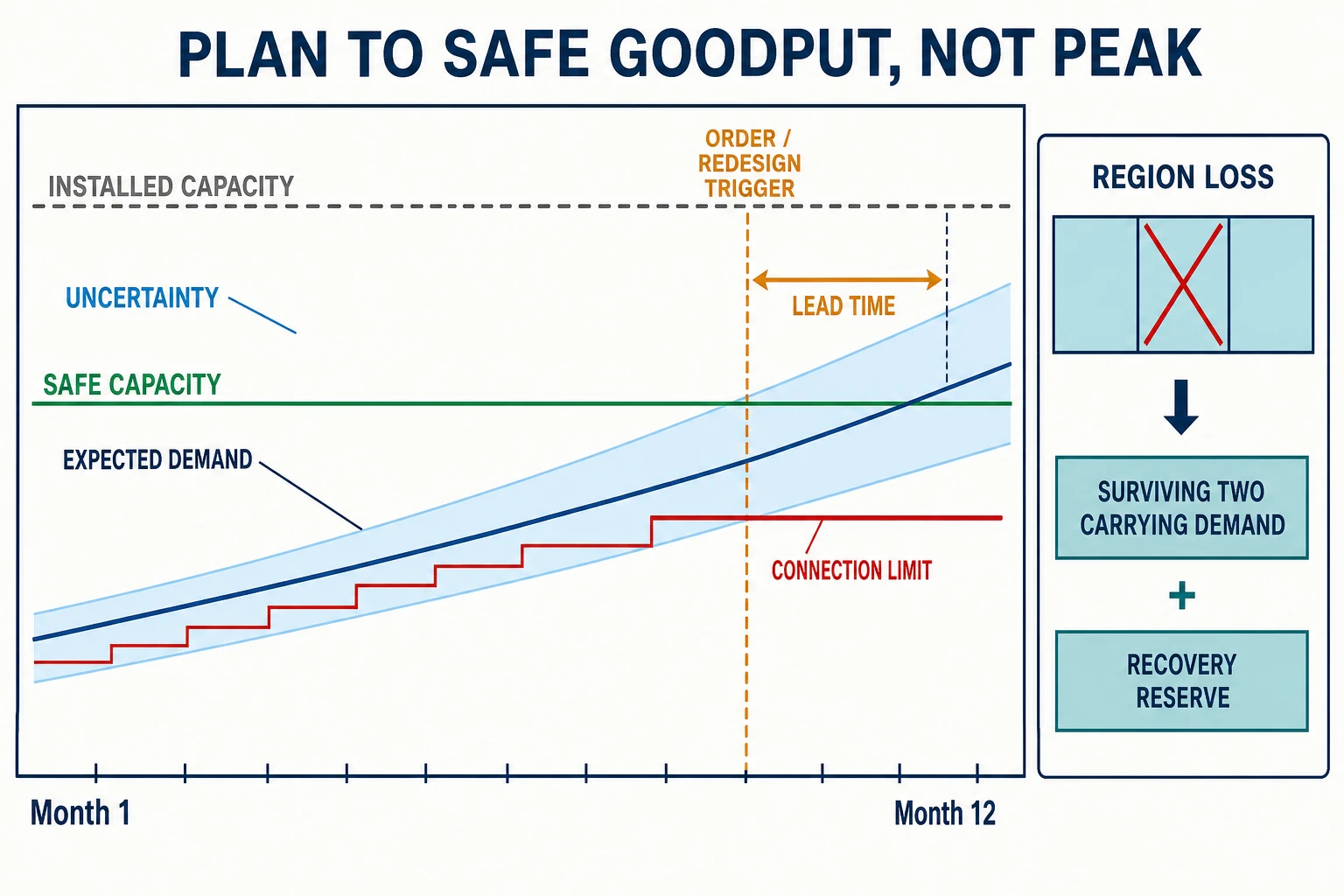
The service must survive one unavailable region while the surviving two carry traffic and reserve work for recovery. It deliberately limits steady CPU occupancy to 65% for the modeled workload and keeps 15% of that surviving service envelope for recovery. Safe compute capacity is therefore 106.08 core-equivalents, not 288. The forecast’s upper planning band crosses that boundary in month 10. A coordinator-connection ceiling crosses in month 8 because a permissions change creates a step increase in connections per query. With three months of procurement or redesign lead time, the earliest action trigger is month 5.
That result is the purpose of capacity planning: expose the first consequential crossing early enough to act. The plan does not predict one exact future. It connects a workload model, measured service demand, uncertainty, failure policy, architecture limits, lead time, and economics to conditional actions. A capacity number without those links is inventory, not a plan.
Define capacity in units that conserve work
“One server” is a procurement unit. It is rarely a stable demand unit. Different operation classes use different CPU time, memory residency, bytes, I/O, locks, connections, accelerators, and downstream work. A fleet can serve fewer requests after the mix shifts even when requests per second is flat.
Choose a normalized capacity unit tied to a conserved resource and a success outcome. For Canopy’s first pass, one core-equivalent means one core-second of CPU service demand per wall-clock second for successful, objective-compliant operations. For operation class i:
D_CPU = Σ_i λ_i S_i
where λ_i is peak arrival rate in operations/s and S_i is measured CPU service demand in core-seconds/operation. The product is core-seconds/s, or core-equivalents.
The month-1 operation ledger is:
| Operation class | Peak rate | CPU service demand | Derived CPU demand |
|---|---|---|---|
| interactive query | 460/s | 0.062 core-s/op | 28.52 cores |
| dashboard refresh | 90/s | 0.180 core-s/op | 16.20 cores |
| export | 2.5/s | 1.400 core-s/op | 3.50 cores |
| Total | — | — | 48.22 cores |
The arithmetic is accounting. Its usefulness depends on the measurements. Service demand must come from representative correct completions, with workload mix, dataset, cache state, runtime version, background work, and saturation state recorded. A service demand measured while a queue is dropping expensive requests can look artificially efficient. A CPU estimate from Chapter 53’s confounded experiment merely scales the confounding.
CPU is only one ledger. Maintain parallel units for the resource paths that can bind first:
- bytes/s and operations/s by storage path, including compaction and rebuild;
- resident and transient bytes by tenant, shard, worker, and cache state;
- concurrent requests, sessions, connections, file descriptors, and stream credits;
- partitions, shards, keys, metadata entries, timers, or queue objects;
- accelerator-seconds, memory bandwidth, network goodput, and cross-domain transfer;
- correct operations/s under the latency objective: safe goodput, not attempted work.
Do not combine them into one arbitrary “capacity score.” Each dimension keeps its units and limit. The plan’s earliest crossing wins unless the architecture can decouple it.
Peak, burst, sustained, and recovery are different contracts
A capacity test should name duration and state:
- Peak demand is the largest relevant workload over a declared interval, such as the busiest five-minute successful-arrival population.
- Sustained demand is load that must be served indefinitely without growing queues, thermal drift, compaction debt, memory retention, or SLO failure.
- Burst demand is a temporary arrival surplus that bounded queues, tokens, or spare workers can absorb and drain before deadlines expire.
- Recovery demand combines user traffic with replay, catch-up, cache warming, repair, rebuild, rebalancing, and reconnect work after a failure.
The distinction changes provisioned capacity. A service may sustain 8,000 operations/s, absorb 12,000/s for 20 seconds, and collapse if 12,000/s lasts five minutes. Another may serve the user peak during region loss but never drain replication backlog, leaving it one fault away from data loss. “Handled the peak” is incomplete until queue age returns to its pre-event band and correctness reconciliation passes.
For every capacity claim, record offered load, correct goodput, latency/error objective, duration, state, resource saturation, backlog at end, and recovery time. Chapter 52’s load and resilience phases supply the evidence; this chapter turns that evidence into installed and safe limits.
Headroom is an explicit failure policy
Headroom is capacity deliberately not assigned to the expected workload. It covers modeled variation and state transitions, not managerial comfort. Name each claim before multiplying percentages:
- demand variance and forecast error;
- deployment overlap or version skew;
- host, rack, zone, or region maintenance;
- one or more failure domains unavailable;
- recovery, rebuild, catch-up, and cache warming;
- imperfect load balance, skew, fragmentation, and unusable small capacity islands;
- measurement uncertainty and guardrail margin.
Percentages should not be stacked blindly. Maintenance and a zone failure may be mutually exclusive by policy, or they may coincide during a real incident. Demand variance may already be represented by an upper forecast band. A rebuild reserve may consume CPU, storage, and network simultaneously. Write scenarios, not a single unexplained “30% buffer.”
Canopy’s compute worksheet is intentionally simple:
| Step | Calculation | Capacity |
|---|---|---|
| installed | 3 regions × 96 cores | 288.00 cores |
| normal utilization envelope | 288 × 0.65 | 187.20 cores |
| N−1 surviving envelope | 2 regions × 96 × 0.65 | 124.80 cores |
| reserve for recovery | 124.80 × (1 − 0.15) | 106.08 safe cores |
The 65% and 15% values are assumptions for this simulated service, not universal targets. A workload with a sharp queueing knee, long garbage-collection pauses, GPU allocation granularity, or high tenant skew may need a different safe point. The right value comes from the resource curve and failure experiment.
N-minus-one must name the “one.” Losing one host is not equivalent to losing a zone, control plane, network path, storage quorum member, or region. Correlated domains matter: two nominal replicas on one power or quota boundary do not provide two units of failure capacity. Map installed resources to failure domains before subtracting.
Forecast the causes, not only the line
A workload forecast should separate at least four components:
- baseline level from a defined recent stable interval;
- trend such as tenant, data, or feature adoption growth;
- seasonality tied to hour, day, month, or known business cycles;
- events and step changes such as launches, migrations, price changes, retention policy, or a new fan-out path.
A smooth extrapolation treats an announced launch as noise and an architectural step as trend. That delays action. Canopy’s multipliers rise gradually through month 6, jump for a launch in month 7, and include a larger seasonal factor in months 11 and 12. Separately, a permissions feature begins in month 6 and holds coordinator connections 15% longer per unit of traffic. The connection step is not CPU growth and must not be hidden inside a fitted line.
Forecast uncertainty should widen with horizon unless contracted facts remove uncertainty. Use a calibrated prediction interval when the data and model justify one; otherwise label a planning band constructed from explicit scenarios. Canopy’s band begins at ±10% and widens to ±30% by month 12. It is modeled scenario uncertainty, not a 95% confidence or prediction interval.
Selected points from the deterministic plan show the decisions:
| Month | Expected CPU demand | Upper planning band | Concurrent coordinator connections | Interpretation |
|---|---|---|---|---|
| 1 | 48.22 | 53.04 | 2,100 | baseline peak model |
| 5 | 60.76 | 69.87 | 2,646 | earliest lead-time trigger |
| 6 | 64.61 | 75.60 | 3,236 | connection step begins |
| 8 | 78.60 | 95.10 | 3,936 | connection safe limit crossed |
| 10 | 88.72 | 110.91 | 4,444 | CPU upper band crosses safe capacity |
| 11 | 107.05 | 135.95 | 5,361 | expected CPU crosses during seasonal step |
| 12 | 113.32 | 147.31 | 5,675 | no-action case is unsafe in both dimensions |
The plan is trigger-based. At month 5, authorize connection-pool redesign or capacity that can complete by month 8. At each monthly review, replace forecast months with actual operation-class rates and measured service demands, recompute bands, and move the trigger only under a documented decision rule. Do not postpone because the point forecast remains below a limit when the accepted risk policy plans against the upper band.
Model error is evidence. Track forecast error by horizon and component: level, mix, trend, seasonality, and event uplift. A consistent high-side error may mean growth is underestimated; alternating seasonal error may mean phase or calendar alignment is wrong; an error only after deployment may be service-demand drift. Replanning should change the causal input, not merely widen every band until alerts stop.
Step functions break linear scaling
Many limits do not degrade smoothly:
- a partition count crosses a coordinator or metadata-memory ceiling;
- a hash table resizes or spills;
- an index no longer fits cache;
- a shard exceeds one device’s rebuild window;
- a protocol field, identifier space, or file-descriptor limit is reached;
- quorum or placement rules require a whole new failure-domain unit;
- connection pools reach the peer’s session or stream cap;
- a dataset exceeds the accelerator or NUMA-local memory boundary.
Canopy permits 2,400 coordinator connections per region and operates to 80% of that during the region-loss scenario. Two surviving regions therefore provide:
C_conn,safe = 2 × 2,400 × 0.80 = 3,840 connections
The month-8 forecast is 3,936, so connections bind while the CPU upper band remains at 95.10 cores, below 106.08. Buying CPU alone does not fix the first limit. The permissions fan-out has changed connection residence time per query; candidates include reducing fan-out, multiplexing, precomputing authorization state, separating long exports, or increasing a verified peer limit with matching memory and failure analysis.
This is why utilization dashboards are not capacity models. CPU can be green while a metadata shard, connection table, queue object count, memory arena, or rebuild clock is red. The workbook needs one row per finite dimension, an owner, an evidence source, a safe limit, current and forecast demand, lead time, and a mitigation.
Storage capacity includes time and repair bandwidth
Storage planning has at least four coupled quantities:
- logical retained bytes after deletion and retention policy;
- physical bytes after replication, coding, indexes, metadata, tombstones, and fragmentation;
- foreground read/write service demand plus compaction, scrubbing, and garbage collection;
- rebuild bandwidth and time under the failure topology.
Canopy’s simulated retained dataset grows from 1.20 PB to 2.10 PB decimal over the horizon. A 48-hour rebuild target for one 2.10 PB region requires a lower-bound transfer rate of:
B_rebuild = (2.10 × 10^15 bytes × 8) / (48 × 3,600 s)
          ≈ 97.2 Gbit/s
That is useful payload before protocol overhead, retries, reads, writes, verification, competing foreground work, and imbalance. If the surviving system cannot reserve that path while meeting user objectives, “48-hour rebuild” is not a target—it is an arithmetic contradiction.
Compaction is a separate write-work multiplier. The fixture assumes 1.8× physical compaction work for a declared interval. Do not multiply the entire stored dataset by 1.8 and call it capacity; apply the factor to bytes entering the compaction boundary under the engine and workload that produced it. Retention changes both stored bytes and background delete/compaction work. A shorter retention policy can temporarily increase work while old data is reclaimed.
Rebuild time is also a risk exposure. A larger shard may reduce metadata overhead but increase the time a failed domain remains degraded. A capacity plan should state maximum unit size, parallel rebuild limit, repair priority versus foreground traffic, checksum/reconciliation work, and the next-failure assumption. Chapter 13 supplies the I/O boundary; Chapters 26 and 27 supply partition and replication semantics.
Elasticity does not create reserved failure capacity
Elastic capacity can match variable demand when resources become available before queues and deadlines fail. It is not instantaneous and not guaranteed. Provisioning, image start, cache warm-up, data movement, connection establishment, load-balancer convergence, quota, regional inventory, and minimum billing or allocation granularity all enter the control loop.
Reserved capacity trades idle periods for predictable availability and often a different price. Elastic capacity trades commitment for responsiveness and flexibility. A robust plan can combine them:
- reserve the sustained demand and the failure capacity that must exist immediately;
- use elastic capacity for forecastable peaks whose provisioning delay fits the objective;
- pre-scale for launches and sharp seasonality;
- maintain quotas, permissions, images, and placement as tested capacity dependencies;
- cap autoscaling so a failing dependency or CPU-burning bug cannot consume the entire budget;
- retain admission and graceful degradation because scaling can arrive too late or amplify a downstream failure.
Autoscaling on CPU alone can be directionally wrong. A dependency stall may hold requests while CPU falls, or a defect may burn CPU without producing useful work. Scale signals should include correct goodput, queue age, concurrency, service demand, downstream saturation, and provisioning/warm-up state. Chapter 36 develops the control-loop design; the capacity plan supplies its feasible envelope.
Reserved and elastic plans must use the same failure scenario. Counting a provider’s nominal regional elasticity as N−1 headroom without quota and availability evidence double-counts hope. Run allocation and scale-out exercises in the domains and time windows that matter, with safety controls.
Lead time turns a crossing into a date
Every mitigation has a delivery distribution:
- quota or purchase approval;
- hardware manufacture, shipping, racking, burn-in, and rollout;
- cloud reservation or regional capacity allocation;
- data rebalancing, index build, or backfill;
- software redesign, correctness review, migration, and rollback;
- contract, licensing, or dependency coordination.
Define the trigger as the first month when an accepted demand bound will cross safe capacity, minus the p90 or otherwise risk-approved mitigation lead time, plus any validation and migration window. If the crossing is month 8 and the end-to-end lead time is three months, month 5 is the last planned start—not the first month to discuss it.
A trigger can be metric-based instead of date-only. Examples include:
- upper six-month demand band exceeds 80% of region-loss safe goodput;
- coordinator connections exceed 75% of safe N−1 slots for three weekly peaks;
- forecast rebuild duration exceeds 36 hours against a 48-hour objective;
- the lower bound of service-demand regression exceeds 8%;
- procurement lead time rises above time-to-exhaustion;
- one tenant or key exceeds the skew reserve.
Use hysteresis and review ownership so normal noise does not repeatedly start and cancel expensive work. A cancellation rule should require new evidence, not a single favorable week.
Capacity risk belongs in a decision register
| Risk | Evidence and threshold | Lead time | Mitigation | Trigger owner |
|---|---|---|---|---|
| coordinator connections under region loss | 3,840 safe; forecast 3,936 in month 8 | 3 months | reduce fan-out, multiplex, or add verified peer capacity | query platform |
| CPU safe-goodput band | 106.08 safe; upper band 110.91 in month 10 | 3 months | add balanced regional cores or reduce service demand | service owner |
| seasonal expected CPU | expected 107.05 in month 11 | 2 months pre-scale | reserve and warm capacity before peak | operations |
| region rebuild bandwidth | 2.10 PB in 48 h needs ≥97.2 Gbit/s useful transfer | 6 months | smaller failure units, more repair bandwidth, or longer approved objective | storage platform |
| service-demand drift | retrigger if any operation class rises >8% with controlled workload | 1 release | regression diagnosis and capacity recalculation | performance owner |
| provisioning uncertainty | p90 allocation time exceeds remaining trigger window | continuous | earlier reservation, alternate domain, admission plan | capacity owner |
The register prevents a forecast from becoming an orphaned spreadsheet. Each row names a finite boundary, evidence, time-to-act, mitigation, and person or team empowered to act. Review it after launches, incidents, topology changes, pricing changes, and forecast misses—not only during annual budgeting.
Price the increment that survives the failure policy
Unit economics should preserve the capacity boundary. A cheap installed core is not cheap if only part of it contributes to safe N−1 goodput.
The next Canopy increment adds 24 cores to each of three regions: 72 installed cores. Under one-region loss, 65% safe utilization, and a 15% recovery reserve, the increment adds:
2 × 24 × 0.65 × 0.85 = 26.52 safe core-equivalents
At an illustrative internal rate of $62 per reserved core-month, the increment costs $4,464/month, or about $168.33 per added safe core-equivalent-month. At $0.118 per elastic core-hour for 730 hours, it costs $6,202.08/month, or about $233.86 per safe core-equivalent-month if held for the whole month. These are modeled internal planning rates, not vendor quotes; quota, commitment, storage, network, support, and engineering work are excluded unless added explicitly.
The calculation changes the comparison. Dividing cost by 72 installed cores would report $62 and $86.14 per core-month while ignoring the failure and utilization policy that made only 26.52 safe units available. The higher safe-unit cost is not waste by definition; it buys bounded behavior under failure and recovery.
Marginal cost also includes the cheapest viable alternative. A software change that reduces interactive-query service demand by 10% saves 2.852 peak cores at month 1 and more as demand grows, but it has engineering cost, delivery risk, and a transfer limit. A connection-fan-out redesign can be economically superior to CPU purchase because CPU is not the binding resource. Compare alternatives at the same objective and failure scenario.
Do not turn utilization into a cost objective by itself. Driving every fleet to 95% can increase queueing, failed work, on-call cost, and emergency capacity premiums. The economic numerator is total cost; the denominator is correct useful work within objectives over the required state envelope.
Operate the model as a living artifact
The machine-readable workbook is examples/performance-engineering-system-design-handbook/part-06/capacity-plan/plan.json. It records operation-class service demand, twelve monthly multipliers and bands, failure headroom, connection limits and the month-6 step, storage/rebuild assumptions, lead time, and modeled economics.
Reproduce the derived demand, crossings, rebuild bound, and marginal increment with:
node examples/performance-engineering-system-design-handbook/part-06/capacity-plan/run.mjs
node examples/performance-engineering-system-design-handbook/part-06/capacity-plan/verify.mjs
A production workbook should add evidence lineage for every input: metric/query or experiment ID, population, aggregation interval, version, owner, date, confidence or scenario label, and transfer limit. Keep actuals immutable, forecast revisions versioned, and assumptions reviewable. A chart without input custody cannot explain why its trigger moved.
At each review:
- reconcile previous forecasts with actual operation mix and outcomes;
- remeasure service demand after material software, runtime, hardware, or topology changes;
- update event, seasonality, and retention assumptions with owners;
- rerun N−1, maintenance, recovery, and skew scenarios;
- scan every finite dimension, not only CPU;
- compare time-to-crossing with updated lead-time distributions;
- execute, continue, narrow, or cancel mitigations under recorded rules;
- update unit economics and budget exposure;
- record residual risks that admission or degradation must contain.
Forecast error should create learning. If expected demand was accurate but required cores were high, the service-demand model changed. If total rate was accurate but connections were high, the operation mix or residence time changed. If normal state fit but region loss did not, the failure model or load balance was wrong. Each error points to a different corrective measurement.
Choose the plan by failure and lead time
| Plan choice | Favor when | Benefit | Cost or risk moved | Decisive evidence |
|---|---|---|---|---|
| reserve sustained and N−1 capacity | capacity must exist immediately under failure | predictable safe envelope | idle normal-state resources and commitment | failure load test, allocation evidence, unit economics |
| combine reserved base with elasticity | peaks are variable but provisioning fits queue tolerance | lower idle allocation | quota, warm-up, control-loop and dependency risk | scale-out distribution, backlog and recovery behavior |
| reduce service demand | repeated work or inefficient path dominates | compounds across future growth | engineering and migration risk | controlled per-class service-demand effect |
| redesign a step limit | metadata, connection, shard, or memory ceiling binds | restores scaling range | architectural correctness and delivery lead time | limit reproduction and new-boundary test |
| shed or degrade | low-priority work can be refused safely | preserves critical goodput | reduced features or rejected work | priority model, correctness, user and recovery objectives |
| accept a scoped risk | mitigation cost exceeds bounded consequence | avoids premature spend | explicit failure or SLO exposure | risk owner, expiry date, monitored trigger and fallback |
Field calculation: rebuild the failure-headroom worksheet
Canopy has three regions with 96 cores each, a 65% measured safe-utilization envelope, and a 15% recovery reserve on surviving capacity. Calculate installed, normal-safe, N−1, and recovery-safe cores. Then compare month 10’s 88.72 expected and 110.91 upper-band core demand. Explain why neither 288 nor 187.20 is the decision boundary. A strong answer identifies 106.08 safe cores, labels the upper-band crossing, and asks whether demand uncertainty and recovery reserve are independent before adding more buffer.
Principal plan revision: launch, retention, and lead-time shock
Build a twelve-month plan from the fixture. After month 4, assume the launch uplift doubles, retention changes from 12 to 18 months, and hardware lead time rises from three to five months. Recompute CPU, connections, stored bytes, rebuild bandwidth, and the earliest trigger. Propose at least two combinations of reservation, service-demand reduction, connection redesign, data placement, admission, and degraded modes. State the cost boundary, failure scenario, migration sequence, rollback, and evidence that would cancel or accelerate the work. There is no single valid architecture; answers fail if they extrapolate CPU alone or move the trigger later without new evidence.
Field checklist
- Are demand units defined by operation class, correct outcome, interval, and state?
- Does every service-demand input have a current, controlled evidence source and transfer limit?
- Are peak, sustained, burst, recovery, and backlog-drain capacities separated?
- Does safe capacity name utilization knee, skew, maintenance, failure domains, and recovery reserve?
- Are trend, seasonality, launches, migrations, and architectural steps modeled separately?
- Is uncertainty a calibrated interval or an honestly labeled planning band?
- Are storage, network, memory, connections, metadata, shards, and quotas forecast beside CPU?
- Does the N−1 scenario identify the actual correlated domain and surviving topology?
- Is time-to-crossing compared with approval, procurement, implementation, migration, and validation lead time?
- Are autoscaling capacity, quota, warm-up, and dependency effects tested rather than assumed?
- Is marginal cost divided by safe useful capacity under the required failure policy?
- Does every risk have an owner, trigger, mitigation, cancellation rule, and expiry?
A forecast is valuable only while there is time to change the system. Plan against correct safe goodput in the states the service must survive, let each finite dimension keep its units, and place action triggers before the uncertainty band reaches the boundary. Chapter 55 will turn these service-demand inputs and resource paths into analytical and queueing-network models; it cannot rescue a capacity plan whose workload, failure state, or limits were never defined.
Sources and evidence scope
- NIST/SEMATECH e-Handbook, Introduction to Time Series Analysis explains why trend, autocorrelation, and seasonal structure matter in time-indexed data. The Canopy planning bands are scenarios, not NIST-derived prediction intervals.
- NIST/SEMATECH e-Handbook, Seasonality describes periodic variation and diagnostic plots used to detect it. A known launch or architecture limit should be modeled as an event or step, not misclassified as seasonality.
- Google SRE Workbook, Managing Load describes autoscaling failure modes, dependency analysis, quota constraints, and bounded scaling. It supports treating elasticity as a controlled mechanism rather than guaranteed headroom.
- Google SRE Workbook, Data Processing Pipelines discusses forecasting growth, allocating capacity, autoscaling variable pipelines, dependency failure, end-to-end objectives, and storage/network cost. Its examples require adaptation to the active system’s workload and failure model.
- Google SRE Book, Addressing Cascading Failures provides operational reasoning about overload, retries, queueing, load shedding, and recovery. Capacity alone does not replace overload control.
- All Canopy operation rates, service demands, multipliers, uncertainty bands, limits, headroom values, storage growth, costs, and trigger dates are simulated teaching evidence in
examples/performance-engineering-system-design-handbook/part-06/capacity-plan/; they are not a vendor quote, cloud limit, production forecast, or observation of this host.