Performance Engineering and System Design Handbook / Chapter 56
Simulation, Trace Replay, and What-If Analysis
Build calibrated, reproducible simulation experiments for transient queues, retries, policies, uncertainty, and feedback that compact analytical models cannot predict.
Preparing audio…
Audio edition
Simulation, Trace Replay, and What-If Analysis
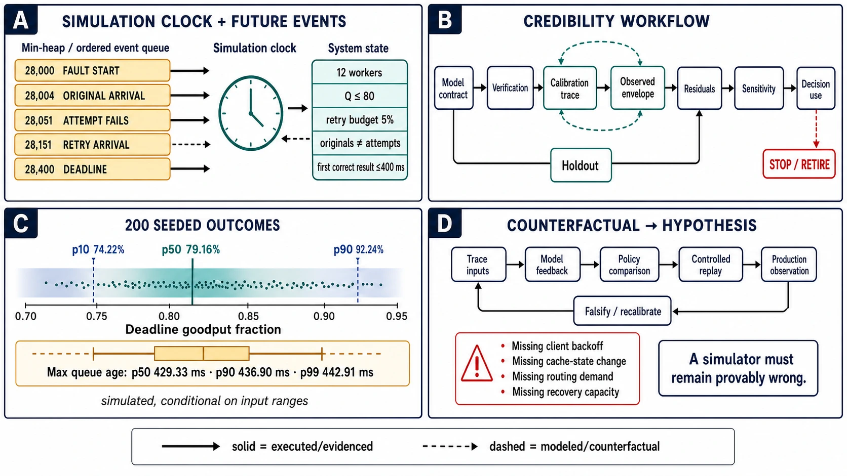
The future-event queue contains five records:
| simulated time | event | state change |
|---|---|---|
| 28,000 ms | dependency fault begins | service multiplier and transient-failure probability enter the declared fault state |
| 28,004 ms | original query 3,781 arrives | offered originals +1; admit, reject, or queue according to policy |
| 28,051 ms | attempt 0 completes with transient failure | worker released; retry eligibility evaluated against identity, deadline, and budget |
| 28,151 ms | retry attempt 1 arrives | attempts +1; original count unchanged; queue policy runs again |
| 28,400 ms | original deadline | later completion consumes work but cannot count as successful goodput |
The simulation clock does not tick through every millisecond. It jumps to the earliest event, applies that event’s state transition, records the consequences, schedules any new events, and jumps again. At 28,051 ms the simulator does not merely draw a red failure dot. It releases a worker, chooses whether to spend retry budget, creates a causally linked attempt, and changes future queue competition. That is the reason to simulate: one policy decision alters the state in which later arrivals are processed.
Chapter 55’s analytical model can still bound service demand, station utilization, and the throughput ceiling. It cannot honestly predict the p95 of this transient from mean station demand once bounded admission, priorities, deadlines, retries, a fault interval, and recovery interact. The next artifact is not a more elaborate spreadsheet. It is an executable claim with a clock, state, inputs, calibration evidence, scenario manifest, and a stop rule.
Simulate only after naming the interaction that matters
Simulation is justified when the decision depends on behavior that a simpler model or controlled calculation cannot represent adequately. Common reasons include:
- nonstationary arrivals, failure, recovery, warm-up, or backlog drain;
- service-time, payload, key, tenant, or fan-out distributions whose tails and mixtures drive outcomes;
- bounded queues, deadlines, cancellation, retries, priorities, batching, routing, caching, or admission policies that change subsequent work;
- state such as cache warmth, device residency, partition ownership, or circuit-breaker mode;
- correlated events and shared failure domains; or
- uncertain inputs whose combined distribution changes the decision.
“The system is complicated” is not a simulation purpose. Write the counterfactual first. Canopy Analytics asks: during the declared spike and dependency fault, which queue and retry policy maximizes correct completions within 400 ms without unbounded waiting or attempt amplification? The output population is original queries. Attempts are tracked separately. The simulator is not asked to reproduce every service or predict next quarter’s incidents.
Use analytical bounds before and after simulation. If service demand gives an absolute ceiling below the target, simulation cannot rescue the design. If a run reports more work completed than worker busy time permits, the implementation is wrong. If a transient result violates Little’s Law assumptions, do not force it through a steady identity; use conservation checks on arrivals, departures, backlog, busy time, and drops instead.
Simulation should be rejected when a direct measurement is cheaper and safer, the decision does not depend on modeled interaction, input evidence is too poor to distinguish alternatives, or implementation detail makes the simulator as hard to validate as the real system. A prototype or bounded load test may provide more credible evidence than months of model elaboration.
A discrete-event clock is a state-transition engine
A minimal sequential discrete-event simulator has:
- a clock representing simulated time;
- a future-event queue ordered by timestamp and a deterministic tie-break;
- explicit state such as workers, queues, capacities, cache mode, failure mode, and retry budget;
- event handlers that mutate state, record outputs, and schedule later events; and
- a deterministic random-number strategy for stochastic inputs.
The core loop is small:
while future_events is not empty:
    event = remove_earliest(future_events)
    accumulate_time_weighted_state(clock, event.time)
    clock = event.time
    apply(event, state, metrics)
    schedule(resulting_events, future_events)
Its semantics are not small. Define the ordering of simultaneous arrival, completion, timeout, failure, and recovery events. If a completion and deadline share one timestamp, does the result count? Does an arrival see capacity released at the same time? Does a fault affect a completion that began before the fault? Different answers can change policy comparisons. Encode the chosen contract and add boundary tests.
Canopy’s fixture uses a binary minimum heap keyed by simulated time and a monotonically increasing sequence. It creates one event for each original arrival. An admitted attempt either starts immediately or enters a bounded queue. Starting schedules a completion based on that request’s service draw. Completion releases a worker, tests the failure state and deadline, records the first successful completion for the original identity, and possibly schedules a retry. Dispatch removes expired queue entries before selecting the next class.
Track time-weighted state correctly. Mean busy workers is not the average of values observed at events; long intervals matter more than short ones. If the previous clock was t_0, the next event is at t_1, and b workers were busy between them, accumulate:
A_b = A_b + b × (t_1 − t_0)
Then divide total worker-time by simulated elapsed time. Apply the same principle to queue depth, cache state, or capacity if their averages support a decision.
Use original identity to prevent a retry from becoming another successful operation in the denominator. Canopy records 8,117 originals, 8,144 attempts, and 6,527 first successful deadline-compliant completions for the bounded budgeted policy. Its amplification is:
A_attempt = 8,144 attempts / 8,117 originals = 1.00333
The simulator must reconcile originals, attempts, retries, queue rejection, expiry, late completion, transient failure, and successful originals. A plausible latency distribution cannot compensate for broken accounting.
Trace replay must preserve the causes of cost
A trace is useful when it preserves production dimensions that drive the decision. Replaying only request counts can destroy exactly the behavior the experiment needs.
For a queue, routing, or cache policy, retain where permitted:
- original timestamp at sufficient resolution and the clock basis;
- logical-operation identity and every attempt’s parent or link;
- operation class, payload or cost shape, key/partition, tenant, geography, and priority;
- deadlines, cancellations, responses, and correctness outcome;
- fan-out or async causal relationships rather than unrelated span rows;
- state markers such as deployment, failure, recovery, cache mode, or topology; and
- sampling, loss, clock-skew, privacy transformation, and missingness metadata.
Preserve inter-arrival gaps when burst shape matters. Preserve complete per-request vectors when branch dependence matters. Preserve key or tenant skew through stable pseudonymous groups when policy allows; shuffling keys into uniform labels invalidates a hot-partition experiment. If timestamps from multiple hosts have uncertainty, retain causal order from parent/child or link relationships and avoid inventing precise cross-host gaps.
Distributed tracing context helps connect spans, but a trace is not a complete execution record. Sampling can omit rare, failed, or long work. Client-side queueing may happen before the first server span. Background compaction, device throttling, and dropped telemetry can change service without appearing as a child span. A trace records what the instrumentation and sampler captured. Its manifest must state the population it represents.
Replay has at least three meanings:
- Arrival replay submits original timestamps and attributes while the simulator or test system recomputes service and outcomes.
- Service replay reuses recorded service draws to compare scheduling or queue policies under common input.
- Full request replay sends captured or reconstructed operations through a real implementation, subject to privacy, side-effect, and safety controls.
Do not mix them silently. Reusing a recorded cache_hit=true while testing a new routing policy bakes the old policy’s outcome into the counterfactual. Reusing recorded service time while claiming to evaluate batching ignores how batch shape changes service. Preserve exogenous inputs; recompute endogenous behavior when the policy can change it.
Canopy’s companion fixture generates a synthetic trace rather than using production data. It preserves original timestamp, class, pseudonymous tenant, original/attempt identity, deadline, service-shape draw, and a deterministic fault draw. That makes policy comparisons reproducible and privacy-safe, but it cannot establish that the chosen distributions match a real service.
Synthetic workloads need mixtures, dependence, and boundaries
Synthetic generation is appropriate when raw traces are unavailable, privacy transformation removes needed detail, future demand lies outside the observed trace, or Monte Carlo scenarios need controlled variation. Fit the dimensions that affect the decision, not every histogram available.
Start with the workload model:
- arrival process by mode and class;
- payload, fan-out, data-set, and operation mix;
- tenant, key, partition, and geography skew;
- service distribution conditional on class, size, cache state, and failure mode;
- dependence between arrivals, shapes, and shared events; and
- growth, spike, failure, and recovery transitions.
One fitted distribution for all service times commonly hides a mixture. An interactive cache hit, interactive miss, and export query can have different mechanisms and tails. Fit or resample classes separately, then reproduce the class mix. A lognormal or gamma-like fit may approximate positive skew for one class, but the name of a distribution is not evidence that it matches the tail or dependence.
Canopy’s teaching generator uses an open arrival process across five declared segments: 90/s nominal, 145/s ramp, 215/s faulted spike, 150/s recovery, and 90/s recovered. Exports are 14% of originals and have 1.9 times the interactive service shape. The faulted segment multiplies service by 1.75, while completions in the first eight seconds of the fault have a simulated 0.18 transient-failure probability. These are model inputs, not observed production facts.
Validate generated data before running policy conclusions. Compare arrival gaps, count variance by window, class mix, conditional payload/service distributions, hot-key concentration, correlations, and extreme clusters against the evidence source. Inspect the quantities the policy sees—queue arrivals, predicted cost, batch compatibility—not only source fields. A generator can match marginal histograms while breaking correlation between large requests and hot tenants.
Rare events require humility. If a one-in-a-million failure mode has no credible mechanism or tail evidence, drawing a million values from a guessed distribution creates precision without knowledge. Use stress scenarios and sensitivity ranges to find failure boundaries. Report them as modeled scenarios, not estimated occurrence frequencies.
Policy simulation is an executable contract review
The same arrival and service draws can compare policy mechanisms under common random inputs. Canopy’s deterministic trace produces:
| policy | queue bound | attempts | retry attempts | success fraction | p95 successful latency | max queue depth | max observed queue age |
|---|---|---|---|---|---|---|---|
| unbounded immediate retry | 5,000 | 8,152 | 35 | 74.36% | 132.54 ms | 125 | 433.42 ms |
| bounded, 5% retry budget, delayed jitter | 80 | 8,144 | 27 | 80.41% | 355.68 ms | 80 | 425.65 ms |
| bounded, no retry | 80 | 8,117 | 0 | 80.14% | 334.13 ms | 80 | 429.53 ms |
All rows use 8,117 original queries and a 400 ms success deadline. “Unbounded” means the teaching policy’s 5,000-entry configuration, not infinite memory. Maximum queue age can exceed 400 ms slightly because expiry is observed when the next dispatch event purges the entry; the work does not start after expiry.
The comparison does not say bounded retry is universally best. In this scenario it recovers 22 additional originals versus no retry, while p95 among successes is 21.55 ms worse and attempts increase by 27. The gain may be too small to justify retries. A product that values early rejection and a tighter successful population could select no retry. A different transient error duration or idempotency contract can reverse the result.
The unbounded row has a counterintuitive p95: it is lower than the bounded rows despite worse goodput. That is survivor bias. Many queued originals expire or complete late and are excluded from the successful-latency population. Reporting p95 of successes alone would make the harmful policy look attractive. Pair latency with original success fraction, deadline miss, rejection, late work, and attempt amplification.
Use simulation to test routing, batching, caching, and admission in the same causal way:
- routing changes which worker, partition, cache, or failure domain serves the request;
- batching changes queue dwell, padding, service, memory, and cancellation;
- caching changes downstream demand, cold-state recovery, and invalidation traffic; and
- admission changes queue state, upstream retries, and useful completion probability.
Each policy needs bounds and an outcome contract. A simulator that queues forever instead of implementing rejection cannot compare overload behavior. A retry model without logical identity cannot measure duplicates. A cache model without cold recovery cannot evaluate failover.
Verification, calibration, and validation answer different questions
Verification asks whether the simulator implements its declared model. Unit tests should cover event ordering, tie behavior, queue bounds, deadline equality, worker release, retry identity and budget, conservation, deterministic seeds, and time-weighted statistics. Compare small cases with hand calculations. Use Chapter 55’s bounds where applicable.
Calibration estimates or selects parameters so declared outputs agree with observed evidence inside a scope. Do not calibrate every coefficient against the final target metric. Use service time, arrival mix, failure duration, cache state, and scheduling evidence directly when available, then compare outputs the fit did not force.
Canopy registers a nominal calibration packet: 30 seconds at 90 originals/s, no fault, and twelve workers. The fixture generates 2,724 originals, all successful, p95 successful latency 98.60 ms, mean busy workers 4.319, and maximum queue depth one. Its teaching envelope expects success fraction 0.997 ±0.015, p95 103 ±18 ms, and mean busy workers 3.9 ±0.8. Passing means the model is not contradicted by those coarse simulated referents. It is not strong validation.
Validation asks whether the model is credible for the decision. Hold out a different time, deployment, tenant mix, region, fault, or input shape. Canopy’s holdout changes the random seed and raises hot-tenant share from 0.38 to 0.52. That only tests skew if tenant identity changes service or routing. In the teaching implementation it does not, so the holdout exposes a model limitation: the simulator preserves tenant labels but lacks a tenant-dependent resource mechanism. A production policy sensitive to hot tenants would fail this validity test until that mechanism is added and calibrated.
Inspect residuals by load, class, tenant, state, and time, as Chapter 55 did. An aggregate match can hide opposite class errors. If predicted queue age is correct at nominal load and wrong in recovery, do not refit one global service multiplier. Add the recovery mechanism or restrict the model’s use.
Separate input uncertainty, parameter uncertainty, stochastic run variation, structural uncertainty, and observation error. Repeated seeds only estimate variability inside the chosen model. They cannot quantify missing mechanisms.
Monte Carlo outcomes are conditional distributions
Monte Carlo analysis runs the simulator repeatedly while sampling declared uncertain inputs and stochastic events. It is useful when the decision depends on a distribution of outcomes rather than one nominal trace.
Canopy’s 200-replication campaign varies three inputs uniformly within registered teaching ranges:
- faulted-spike arrival multiplier: 0.90–1.12;
- fault-state service multiplier: 1.55–2.05; and
- transient-failure probability: 0.10–0.24.
For the bounded budgeted policy, the simulated success-fraction distribution is:
| outcome quantile across replications | success fraction |
|---|---|
| p10 | 74.22% |
| p50 | 79.16% |
| p90 | 92.24% |
The maximum observed queue-age distribution has p50 429.33 ms, p90 436.90 ms, and p99 442.91 ms. These quantiles describe simulator outputs under the specified input distributions and seed scheme. They are not confidence that production lies in the interval. A uniform input range encodes an assumption that must have evidence or be labeled exploratory.
Use independent random streams or stable keyed draws so policy comparisons share arrival and service randomness without accidentally changing one policy’s inputs after a different number of random calls. Record seeds and generator version. Run enough independent replications for the decision metric to stabilize, and show the convergence check. If estimating a very low probability, ordinary Monte Carlo may require impractical samples; importance sampling or targeted stress analysis needs specialist design and independent validation.
Sensitivity should vary coherent scenarios, not only one coefficient at a time. A region failure may raise routing distance, cold misses, service demand, retries, and offered load together. Preserve those relationships. Factorial or space-filling designs can expose interactions more efficiently than an undirected grid, but the ranges and dependencies still require justification.
The decision should survive plausible uncertainty. If two policies exchange rank across credible ranges, the simulation has identified the next measurement or a need for a robust policy, not a winner.
One historical trace is one realized world
Overfitting occurs when the simulator reproduces one trace’s incidental order, mix, topology, or failure and is treated as a general system model. A policy can look excellent because the trace happens to contain no aligned tenant bursts, no long request before a priority inversion, or one favorable cache state.
Protect against this by using:
- multiple traces from different time blocks, modes, regions, deployments, and workload mixes;
- a calibration/holdout split based on independent operational units, not random rows from one burst;
- resampling complete causal groups rather than independent spans;
- synthetic stress cases that vary the dimensions the trace did not exercise;
- mechanism-specific invariants and conservation tests; and
- explicit transfer limits for topology, version, state, and range.
Time scaling is especially dangerous. Compressing a one-hour trace into six minutes multiplies arrivals by ten, but background timers, cache expiry, connection reuse, autoscaling, quota periods, and client think time may not scale. If those clocks stay fixed, the experiment is a new workload, not a faster replay. State which clocks and rates change and why.
Trace privacy transformations can also alter performance structure. Hashing stable keys may preserve popularity; replacing every key with a random token does not. Bucketing payloads may preserve size classes while removing a boundary condition. Removing rare tenants can erase the very skew a fairness policy needs. Treat the transformed trace as a new dataset with its own validation.
Counterfactuals fail where feedback is frozen
A counterfactual asks what would have happened under a policy that did not generate the observed trace. Historical replay cannot answer when the policy changes future inputs or service.
Four Canopy feedbacks are explicitly absent from its fixed trace:
- client backoff changes future offered arrivals after rejection;
- routing changes cache locality and therefore service demand;
- admission changes upstream concurrency and timeout behavior; and
- recovery changes cache warmth and available worker capacity.
If a replay feeds the same attempts into every admission policy, it can compare local queue mechanics but not client-system equilibrium. Add a client model calibrated from rejection/backoff behavior, run a controlled experiment, or limit the claim. If routing moves a tenant, recompute cache hits and partition service rather than replaying old service times. If a cache policy changes hit/miss state, model object identity, capacity, admission, invalidation, and cold recovery.
Missing organizational and operational feedback matters too. Operators may shed a feature when queue age crosses a threshold. Autoscaling has detection and provisioning delay. A rollback changes workload and state. A digital control loop that never appears in the simulator can dominate the incident.
Counterfactual language should be conditional: “Under the declared arrival, service, fault, and client-response model, policy B produced more deadline goodput than policy A.” The next sentence should identify what production evidence can falsify it.
Speed and scenario management are part of credibility
A slow simulator discourages replication, sensitivity, and review. Profile the simulator separately from the system it models. Use an appropriate event queue, avoid per-tick work in sparse-event systems, aggregate only when it preserves the decision, and provide a smaller deterministic verification suite. Parallel replication is usually simpler than parallelizing one event clock; shared state and event ordering make the latter a semantic as well as performance problem.
Optimization must preserve outputs. Compare event counts, state trajectories, and registered summary metrics against a trusted small implementation. A faster simulator that changes simultaneous-event order has changed the model.
Every experiment needs a manifest:
| field | Canopy record |
|---|---|
| decision | choose queue bound and retry policy during spike plus transient fault |
| boundary and unit | original query at gateway through first correct completion; attempts separate |
| success | first correct result within 400 ms |
| evidence and data | simulated generated-trace specification; no production data |
| versions | model des-fixture-1; dependency-free ECMAScript module; runtime recorded at execution |
| workload | five arrival/service modes, class mix, tenant labels, deadline, twelve workers |
| policies | queue bound, priority, retry count, delay/jitter, and retry-budget fraction |
| failure/recovery | fault window, service multiplier, transient failure, recovery segment |
| seeds/replications | base seed 560016; 200 uncertainty replications |
| outputs | success fraction, successful p95, attempts, queue depth/age, busy workers |
| calibration/holdout | nominal envelope; different seed and hot-tenant share |
| stop rule | calibration miss or policy activates an unmodeled feedback/service mechanism |
| transfer limit | teaching model; no production, rare-event, or live-control guarantee |
Store scenario inputs, seeds, source revision, environment, output schema, and raw or reproducible results together. Give scenarios stable names and immutable versions. A changed queue policy under the same scenario version is difficult to audit. Keep exploratory runs separate from decision evidence.
Treat “digital twin” as a claim with an update contract
A live or periodically synchronized model may be useful for capacity, routing, maintenance, or anomaly analysis. The label digital twin does not increase credibility. Ask:
- Which physical or software state is represented, at what boundary and resolution?
- Which inputs update continuously, which are inferred, and how stale may they be?
- Which mechanisms and control loops are absent?
- How are version and topology changes detected?
- Which outputs are validated, against what holdout evidence and tolerance?
- What happens when residuals exceed the acceptance boundary?
- Is the model advisory, or can it change production state?
An advisory what-if model and an automated controller have different safety obligations. A controller needs fail-safe limits, authorization, rollback, monitoring, and an independent operating envelope. No simulator should gain actuation authority merely because its inputs are current.
Retire or quarantine a simulation when calibration fails, workload or topology leaves range, a new policy changes an unmodeled feedback, missing telemetry prevents causal reconstruction, output sensitivity is dominated by unsupported assumptions, or a direct production test contradicts it. Use history as evidence, not as reputation.
Convert results into a testable production hypothesis
A simulation result should end in a discriminating experiment. Canopy’s packet can produce this hypothesis:
Under a controlled replay of the registered spike and dependency-delay envelope, an 80-entry gateway queue with one delayed jittered retry under a 5% retry budget will preserve at least six percentage points more original deadline goodput than the current large immediate-retry queue, while attempt amplification remains below 1.01.
The test must then specify representative originals, open-loop arrival schedule, generator validation, dependency fault, queue/retry configuration, original/attempt identity, correctness oracle, deadline, abort criteria, and recovery observation. Measure success fraction, queue age, attempts, late work, and p95 for the same population. Preserve raw observations and compare residuals with the simulator.
Do not test only the favored policy. Run a control and at least one alternative under blocked/randomized repetitions. If the gain is smaller, inspect whether input mismatch, implementation mismatch, or missing feedback explains it. If the result remains useful but differs in magnitude, recalibrate. If the mechanism is wrong, retire the model.
Simulation reduces the cost of asking better questions. The controlled test decides whether its answer transfers.
Field exercise: audit the Canopy campaign
Run node run.mjs and node verify.mjs in examples/performance-engineering-system-design-handbook/part-06/simulation-what-if/, then:
- reconcile originals, attempts, retries, successes, rejections, expiry, late completion, and transient failures for each policy;
- explain why successful p95 makes the unbounded policy look better than its success fraction does;
- decide whether the 0.27 percentage-point gain of budgeted retry over no retry justifies retry complexity;
- identify the simultaneous-event ordering rule the fixture uses and write one boundary test for deadline equality;
- distinguish verification, calibration, holdout validation, and Monte Carlo replication in the package;
- explain why the hot-tenant holdout is weak in this model; and
- write the smallest controlled load test that could falsify the bounded-policy hypothesis.
A strong audit may select no retry. The exercise assesses evidence boundaries, not agreement with the chapter’s provisional policy.
Principal drill: find the counterfactual that cannot be replayed
Canopy now routes hot tenants to isolated workers, maintains a result cache whose keys migrate with routing, scales after 30 seconds of queue-age burn, and sends retry hints that some clients honor with jitter while others retry immediately. During region loss, cache warm-up and exports compete for the same database partitions. The team provides one sampled trace from a healthy region and requests p99 recovery predictions.
Produce four lists:
- Replayable evidence: exogenous timestamps, operation shapes, causal groups, tenants, deadlines, and state markers the trace genuinely preserves.
- Required model: client response, routing/cache state, autoscaling delay, failure capacity, recovery traffic, class scheduling, and database service under skew.
- Required experiments: calibration runs, holdout region/failure campaign, client-behavior measurement, cache-cold replay, and controlled recovery test.
- Invalid claims: any p99, region-loss, rare-event, or digital-twin conclusion unsupported by the one trace and missing loops.
Then write a scenario manifest, three conservation/ordering tests, one uncertainty campaign, one stop rule, and one production hypothesis. Keep Chapter 55’s bottleneck and service-demand bounds even though response prediction moves into simulation.
Evidence and transfer limits
- Berkeley’s Ptolemy II discrete-event modeling report describes event-queue ordering, simulation time, and deterministic handling of simultaneous events in a rigorous discrete-event domain. Canopy is a small independent implementation, not Ptolemy.
- NASA-STD-7009B, Standard for Models and Simulations defines current credibility practices across a model’s development and use, including verification, validation, uncertainty, sensitivity, and acceptance criteria. This chapter adapts that discipline to performance decisions; it does not claim NASA accreditation.
- NIST’s statistics guide for verification and validation of simulations emphasizes experimental design, calibration referents, uncertainty, and prediction error. The NIST engineering statistics glossary defines Monte Carlo sampling as random-number computer experiments for simulator-output distributions.
- W3C Trace Context standardizes propagated identifiers for distributed tracing. It provides correlation context, not complete causality, timing accuracy, or sampling coverage.
- OpenTelemetry’s trace specification defines spans, parents, links, timestamps, events, and status; its overview explains causal span graphs and links for batched or async work. Instrumentation still determines what is recorded.
- All Canopy inputs and outputs are simulated teaching evidence reproduced by
examples/performance-engineering-system-design-handbook/part-06/simulation-what-if/. Passing checks proves implementation identities and reproducibility, not production validity.
The decision rule is: simulate when distributions, transient state, and policy feedback drive the outcome; trust a counterfactual only after the implementation is verified, inputs are calibrated, outputs survive independent validation and sensitivity, and a controlled observation can still prove it wrong.
Chapter 57 turns that final observation into a continuous validation system. A simulation that cannot be versioned, rerun, compared, and retired is not a regression control; it is an anecdote with code.