Performance Engineering and System Design Handbook / Chapter 53
Experimental Design and Performance Statistics
Design controlled performance comparisons that separate useful effects from host variation, workload drift, metric fishing, and stopping bias.
Preparing audio…
Audio edition
Experimental Design and Performance Statistics
The proposed allocator is “5% faster.” The result packet contains two bars, one number above each bar, and no raw runs. Build A ran on four newly provisioned hosts in the morning. Build B ran on four older hosts after the load generator had warmed the data set. Failed operations were omitted. The team stopped after the first dashboard refresh that showed a favorable difference.
The arithmetic may be correct and the claim still unusable. Host, time, cache state, workload, outcome selection, and stopping have all changed with the treatment. There is no defensible counterfactual—no answer to what the same experimental units would have done under the other allocator. “5%” names neither an effect population nor its uncertainty, and it says nothing about whether the difference matters to the system objective.
Statistical machinery cannot repair an undefined comparison. The engineering sequence is: state the decision, define the effect, assign treatments so alternatives are comparable, preserve the run structure, quantify uncertainty, inspect threats and guardrails, and then decide. This chapter supplies that sequence. It is not a catalogue of tests, and it does not turn observational telemetry into causality by adding a regression line.
Define the claim before collecting a run
An experiment begins with an estimand: the exact effect the analysis intends to estimate. For a performance change it could be the mean paired percentage reduction in median request latency for correct operations, under a declared warm workload and host population. It could instead be the change in correct goodput at a fixed latency objective, a p99 non-inferiority bound, or bytes allocated per completed operation. These are different decisions.
Write the claim in five parts:
- Population: workloads, hosts, versions, operating state, time, and outcomes to which the result should transfer.
- Experimental unit: the independently assigned unit that could receive either treatment.
- Treatment and counterfactual: what changes and what the same unit would have experienced otherwise.
- Outcome and effect: metric population, summary, direction, and comparison scale.
- Decision threshold: the smallest operationally useful improvement and any non-regression guardrails.
Requests emitted inside one benchmark process are rarely thousands of independent experimental units. They share a binary, host, cache, allocator state, kernel, clock, background work, and run order. Treating every request as independent produces a huge nominal sample while leaving only one deployment or host comparison. The experimental unit is often a host deployment, process, run window, tenant cell, or time block.
The unit determines what replication means. Repeating a request inside one run estimates within-run variation. Restarting the process samples initialization and address-layout effects. Rebuilding samples compilation variation. Repeating across hosts samples host variation. Repeating over days samples environmental drift. More observations at the wrong level do not substitute for replication at the level of the claim.
Design controls create a counterfactual
Let Y_i(A) and Y_i(B) denote the outcome experimental unit i would produce under allocators A and B. Only one treatment can usually be observed at a moment; the missing potential outcome is the counterfactual. Experimental design makes the observed alternative credible enough to estimate the difference.
Three controls do different work:
- Randomization uses a declared random process to assign order or treatment, breaking systematic alignment with known and unknown nuisance factors in expectation.
- Blocking groups units that share a strong nuisance factor, such as host class, region, data snapshot, or time window, so treatment is compared within those groups.
- Pairing applies both treatments to closely matched or the same reset unit, then analyzes within-pair differences rather than unrelated group totals.
Repeated measures reuse a unit across treatments or times. They can be efficient because stable unit differences cancel. They also introduce dependence, carryover, warm-up, fatigue, cache contamination, and time trends. The analysis must preserve the pairing or repeated structure; pretending the observations are independent discards the design and misstates uncertainty.
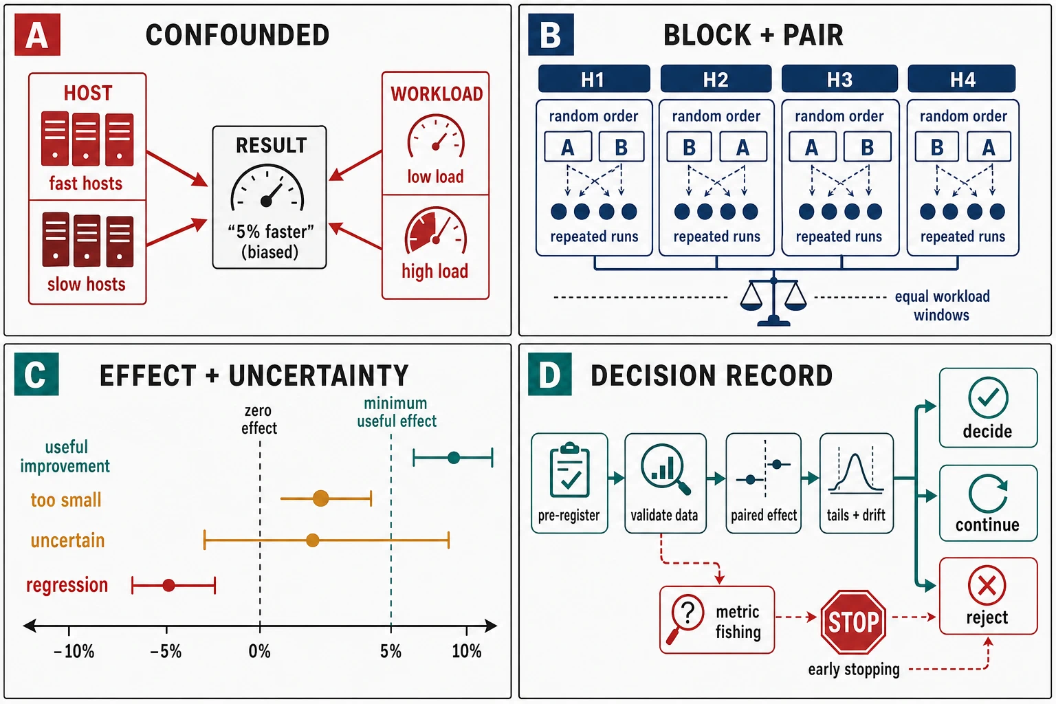
For the allocator experiment, use four host blocks. On every host, run A and B with the same deployment image, data snapshot, offered-load target, and reset protocol. Randomize whether A or B runs first within each repetition. Repeat three pairs per host. This design estimates treatment differences within hosts and exposes treatment-by-host variation instead of rewarding whichever version received faster machines.
Blocking does not justify silently narrowing the population. Four hosts from one hardware family in one lab session support that environment. They do not establish behavior across other processors, kernels, allocators, regions, cold starts, traffic mixes, or month-long drift. Generalization requires sampling or separate validation across those dimensions.
A baseline is not automatically a counterfactual
“Before” is attractive because it already exists. It is also entangled with everything that changed after it: workload, tenancy, cache state, deployment image, dependency behavior, host placement, seasonality, and observability. A baseline is a useful reference; it becomes a credible counterfactual only when the design controls the competing changes well enough for the claim.
An A/B experiment assigns comparable units concurrently or in a controlled sequence. Request-level assignment can balance time and workload quickly, but it may violate isolation: both variants can share caches, queues, connection pools, locks, or downstream limits. Host- or cell-level assignment reduces some interference but yields fewer independent units and can expose host imbalance. Tenant assignment may preserve user journeys while introducing tenant-size skew.
A canary is usually selected for rollout safety, not random inference. It may receive a small region, one cluster, volunteer traffic, or a lower-risk tenant set. Its result is operational evidence for that slice. Calling it an A/B test does not make the control population exchangeable. If causal comparison matters, randomize eligible units or use an explicitly justified quasi-experimental design and weaken the claim.
The baseline also needs a state policy. A warm candidate compared with a cold control answers a warm-versus-cold question. A new allocator that inherits the old allocator’s fragmented heap measures a migration state. Resetting everything may remove the production transition that matters. Pre-register cold, warm, steady, degraded, and recovery populations separately.
Effect size and uncertainty answer different questions
An effect size expresses the magnitude of a comparison. For latency, useful choices include an absolute difference in milliseconds, a ratio, or a percentage reduction. Ratios need a direction convention. This chapter defines paired reduction for pair i as:
r_i = 100 × (A_i − B_i) / A_i
where A_i and B_i are the same declared latency summary in milliseconds for one valid pair. A positive r_i means B is faster. The formula is undefined for a zero baseline and can behave asymmetrically for large changes; preserve the original units alongside it.
Uncertainty describes how much the estimate would vary under the sampling and assignment process represented by the model. A frequentist 95% confidence interval is produced by a procedure that would cover the target parameter in 95% of repetitions under its assumptions. It is not a 95% probability that this one fixed interval contains the effect. The assumptions—independence at the experimental-unit level, design, distributional approximation, and stopping rule—matter more than the label.
For n paired reductions, the teaching interval in the fixture is:
mean(r) ± t_(0.975,n−1) × s_r / √n
where mean(r) is the mean paired reduction in percent, s_r is the sample standard deviation across paired experimental units, and n is the number of valid pairs. This interval summarizes between-pair uncertainty for the modeled design. It is not automatically appropriate for a skewed ratio, dependent time series, adaptive test, or hierarchical fleet without further work.
Practical significance asks whether the effect is large enough to change an engineering decision. If allocator migration costs four engineer-weeks and the end-to-end objective needs at least a 3% latency reduction, an interval of 0.1% to 0.3% may be precise and statistically nonzero but operationally irrelevant. Conversely, an interval of −1% to 9% contains a valuable improvement and a regression; the answer is not “no effect,” but “insufficient precision for this decision.”
The American Statistical Association’s p-value statement makes the corresponding warning explicit: a p-value does not measure effect size or importance, and decisions should not depend only on passing a threshold. Report the estimate, interval, design, raw units, threshold, guardrails, and threats.
Work the paired allocator result without hiding the tails
The retained fixture contains twelve simulated paired units: four hosts × three repetitions. A/B order is balanced within host repetitions. Offered load stays within 6,970–7,030 operations/s, and cache-miss share stays within 7.8%–8.2%. Every run is warm and uses the same declared data snapshot and deployment image.
The paired median-latency reductions produce:
- mean reduction: 4.83%;
- teaching 95% interval: 4.75% to 4.91%;
- predeclared minimum useful effect: 3%;
- valid paired experimental units: 12.
The pairing remains visible by host instead of disappearing into two fleet bars:
| Host block | Mean A median | Mean B median | Mean paired reduction | Pair range |
|---|---|---|---|---|
| H1 | 101.00 ms | 96.17 ms | 4.79% | 4.65%–4.94% |
| H2 | 107.93 ms | 102.67 ms | 4.88% | 4.74%–4.99% |
| H3 | 94.07 ms | 89.50 ms | 4.85% | 4.68%–5.01% |
| H4 | 115.00 ms | 109.47 ms | 4.81% | 4.71%–4.94% |
The absolute host levels vary by more than 20 ms, while the within-host reductions remain close. That is the result the blocked paired design was built to expose; an unpaired fleet average would mix host composition into treatment.
The lower interval bound exceeds the useful-effect threshold, so the primary usefulness gate passes for this simulated population and model. That is stronger than “the point estimate is about 5%” because it states what varied and how precisely the paired effect was estimated.
It is not yet an unconditional adoption decision. Allocator B has a higher per-run p99 in three of twelve pairs, while the pre-registration says adoption requires no p99 regression but fails to define a tail non-inferiority margin, aggregation method, or uncertainty procedure. Counting directions preserves the warning; averaging the twelve p99 values would be invalid because percentiles from separate run populations do not combine into a fleet percentile. The experiment contract needs a predeclared p99 estimand—perhaps a bound on the ratio of per-run p99 values or a pooled raw-latency quantile under a justified population—and a practically acceptable margin.
This is a valuable failure of pre-registration, not permission to invent a favorable tail rule after seeing the results. The defensible report says: primary median effect passes; correctness and goodput remain guardrails; tail non-inferiority is unresolved because the decision rule was underspecified; run a confirmatory tail analysis or experiment before adoption.
Run the deterministic analysis with:
node examples/performance-engineering-system-design-handbook/part-06/controlled-experiment/run.mjs
node examples/performance-engineering-system-design-handbook/part-06/controlled-experiment/verify.mjs
The interval’s narrowness is intentionally simulated to teach interpretation. It must not be presented as observed allocator evidence.
Compare distributions at the decision boundary
Means and medians compress a population differently. A lower median can coexist with a worse p99 if a treatment speeds the ordinary path but adds a rare slow path. A throughput increase can coexist with fewer correct completions if retries or failures are counted as work. Choose the distribution and outcome population from the objective.
For request latency, preserve raw observations or mergeable histograms with compatible boundaries and sufficient precision. Segment correct, failed, timed-out, cancelled, and in-flight-at-end outcomes. Define whether the latency begins at intended arrival, client send, server admission, or service start. A server-side p99 cannot establish a client deadline if queueing and network time are outside it.
Tail comparison needs enough observations at the experimental-unit level and a method suited to quantiles. “One million requests” is not one million independent deployments. Run-to-run variation can dominate within-run quantile error. Report both: uncertainty in each run’s tail estimate and variation across valid runs or blocks. If the decision concerns a maximum or extreme tail beyond the sample’s reliable rank, state that the experiment cannot estimate it.
Distribution plots can reveal bimodality, truncation, changing failure populations, and phase mixtures that one quantile hides. Align axes and show per-block or per-phase views. A smoothed aggregate that blends warm-up, steady state, fault, and recovery creates a distribution that no operating state actually experiences.
Metric fishing spends credibility
A dashboard with 200 metrics offers many opportunities for one favorable change. If the team tries every endpoint, percentile, time window, host subset, normalization, and exclusion rule and reports only the best, the nominal uncertainty no longer describes the selection process. This is metric fishing or multiple-comparison selection.
The remedy starts before correction formulas:
- name one or a small family of decision metrics;
- declare guardrails and their margins;
- predefine slices required by the workload model, such as operation class or tenant tier;
- label all unplanned slices exploratory;
- confirm an exploratory finding on new data;
- report the analysis family and negative results, not only the winner.
Multiplicity adjustments can control a chosen error rate for a declared family, but they cannot rescue arbitrary post hoc transformations or undisclosed exclusions. The engineering goal is not the smallest p-value. It is a stable, useful effect that survives the workload and failure envelope.
Secondary metrics are still essential for mechanism. Allocated bytes, CPU service demand, cache misses, pause time, and correct goodput can explain why latency moved. Treat them as diagnostics unless the decision contract assigns them a gate. A diagnostic association supports a hypothesis; it does not silently become a second success criterion.
Time can masquerade as treatment
Performance environments are nonstationary. Traffic grows, caches warm, data compacts, tenants shift, hosts throttle, dependencies deploy, and daily or weekly cycles change the population. If all A runs precede all B runs, any trend is perfectly confounded with treatment.
Randomized order spreads simple time effects. Blocking by hour, day, host, or data snapshot keeps close comparisons together. Pairing can reduce slow drift when the pair duration is shorter than the drift timescale. None of these controls helps if A changes the state inherited by B and reset is incomplete. Use washout, independent environments, or a model of carryover.
Plot outcomes against run order before collapsing them. Record offered load, operation mix, hot-key share, cache state, background work, thermal or frequency state, and dependency indicators. A flat total rate can hide a growing expensive-operation share. Chapter 52’s phase boundaries remain part of the data; do not treat recovery samples as ordinary steady state.
Seasonality is a repeated temporal pattern. One lab afternoon cannot validate a weekly production effect. Workload drift changes the distribution being served. A reweighted analysis can estimate what would happen under a target mix only if all material strata are observed with adequate support. Extrapolating beyond the measured range is a model claim, not experimental evidence.
Outlier policy is a data-quality contract
An outlier can be a measurement error, an unrelated interruption, or the system’s most important slow path. Deleting it because it is inconvenient biases the result. Decide exclusions without using the treatment outcome whenever possible.
The fixture invalidates a run only for a correctness failure, generator schedule loss above 1%, thermal throttling, or missing required telemetry. These conditions mean the intended experiment was not executed or cannot be interpreted. The raw run remains in custody with an invalidation reason. A high but valid latency does not qualify.
For surprising valid observations:
- inspect raw timestamps, units, clocks, and population membership;
- find a mechanism such as fault, checkpoint, retry, or queue burst;
- report the primary analysis with the observation;
- add a labeled sensitivity analysis when justified;
- repeat under a predeclared discriminating condition.
Winsorizing, trimming, or robust summaries can be valid for a specified estimand. They are not generic cleanup. State what population the transformed result represents and what operational tail it may suppress.
Looking repeatedly changes the stopping process
Suppose a fixed-horizon test plans twelve pairs but checks after every pair and stops the first time a conventional interval excludes zero. The chance of a favorable random excursion is no longer the fixed-horizon error rate. Stopping on an extreme also tends to exaggerate the observed effect at that moment.
Two honest strategies are available. Use a fixed sample or precision rule and do not make inferential decisions at unplanned looks. Or use a sequential design whose interim schedule, stopping boundaries, error spending or evidence threshold, effect estimator, and maximum sample are declared in advance. Sequential analysis is a designed method, not permission to refresh until green.
Safety stopping is separate. Stop immediately for correctness loss, blast-radius breach, or harmful user impact regardless of inferential efficiency. Record that the performance comparison was truncated and use analysis appropriate to the stopping event. Protecting the system takes precedence over completing a balanced table.
The allocator fixture uses a fixed twelve-pair rule. If the interval is too wide at the end, “continue until significant” changes the design. Pre-register a precision-based extension rule—for example, add one balanced repetition to every host up to a maximum—using a method whose coverage accounts for that rule.
Regression adjustment can improve precision, not invent assignment
A regression model can account for measured workload differences:
latency = treatment + host block + offered load + cache-miss percentage + residual
In a randomized blocked experiment, this adjustment may improve precision and describe heterogeneity if the form is credible. Preserve the assignment and dependence structure in standard errors or hierarchical terms. Check residuals, influential blocks, nonlinearities, interactions, and overlap in covariates.
Adjustment does not make an observational comparison randomized. If treatment B ran only at lower load, the model must extrapolate treatment at high load. If an unmeasured background job affected only B, no coefficient for offered load removes it. If treatment changes cache-miss rate, controlling for that mediator can remove part of the effect the experiment intended to measure. Draw the causal story before selecting covariates.
Predeclare adjustment covariates that improve precision, and report both adjusted and design-consistent unadjusted estimates where useful. A large disagreement is diagnostic evidence about imbalance, model form, or data quality—not a menu from which to choose the better result.
Change points detect candidates, not causes
A performance series may shift after a deployment, dependency change, workload event, or measurement revision. Change-point methods search for times at which distributional parameters change. They can detect a candidate boundary more consistently than eyeballing a chart, but the selected point is not a causal label.
A regression-prevention workflow should:
- preserve comparable per-commit or per-window experimental units;
- detect a sustained level, slope, variance, or distribution change using a predeclared method;
- account for seasonality, missingness, infrastructure migrations, and repeated looks;
- inspect changes and mechanisms near the boundary;
- reproduce the candidate in a controlled comparison;
- update the baseline only after the new state is understood.
Binary search or commit bisection is powerful when builds are reproducible and the effect is monotonic across revisions. It fails when one change requires another, infrastructure drift dominates, or the metric is too noisy. A change point narrows the search; Chapter 57 turns that evidence into a regression gate.
Communicate uncertainty as a decision range
Uncertainty does not require paralysis. It requires conditional language tied to action:
- Adopt: the effect interval exceeds the useful threshold, guardrails pass, and transfer covers the rollout population.
- Reject: the interval rules out a useful effect or shows an unacceptable regression.
- Continue: the interval includes materially different decisions and another balanced sample can reduce uncertainty at acceptable cost.
- Narrow: the effect is supported only for a workload, host, or phase where a scoped rollout creates value.
- Redesign: confounding, invalid units, data loss, interference, or an undefined guardrail prevents interpretation; more of the same data will not help.
Lead the report with one of those dispositions. Then show effect and interval in original and relative units, practical threshold, primary and guardrail outcomes, experimental units and assignment, exclusions, raw-data path, diagnostics, sensitivity, transfer limits, and residual risk. Do not average a red correctness gate with a green latency gate.
Pre-register the engineering degrees of freedom
The machine-readable template at examples/performance-engineering-system-design-handbook/part-06/controlled-experiment/experiment.json contains a filled allocator example. A reusable pre-registration should include:
| Field | Required decision content |
|---|---|
| decision and owner | action the evidence can authorize; risk owner |
| population and boundary | workload, environment, versions, state, time, outcomes |
| experimental unit | independent assignment/repetition level |
| treatment/counterfactual | exact change and comparator |
| estimand | effect, direction, units, population summary |
| primary metric | measurement boundary and success/failure inclusion |
| useful threshold | minimum effect that changes the decision |
| guardrails | correctness, p99, goodput, cost, recovery, with margins |
| assignment | randomization unit, blocked factors, pairing, order |
| state control | reset, warm-up, carryover, data snapshot, background work |
| sample/stopping | fixed or sequential design, looks, maximum, safety stops |
| data quality | clock, generator, telemetry, invalidation and missingness rules |
| analysis | interval/model, dependence, multiplicity, tails, sensitivity |
| drift | run-order plots, trend/seasonality coverage, workload adjustment |
| custody | raw runs, manifest, code, deviations, exploratory analyses |
| transfer | environments and states the result does not cover |
Pre-registration is not bureaucracy for its own sake. It prevents the result from deciding which question was supposedly asked. Deviations are allowed when the system teaches something unexpected; record them and label the resulting analysis exploratory.
Field review: critique “5% faster”
You receive 200,000 request samples per variant, one host per variant, unknown run order, a 5% median difference, no failed operations, and no workload or cache-state record. Write a decision report. Identify the experimental unit, confounders, missing population rules, minimum useful effect, and tail/correctness guardrails. Design the smallest controlled rerun that could support a scoped decision. A strong answer does not treat request count as host replication and does not claim “no effect” merely because uncertainty cannot be computed.
Principal experiment: compare allocators across variable hosts
Design the A/B allocator experiment for four heterogeneous hosts, three workload mixes, warm and post-restart states, and a p99 non-inferiority requirement. Specify blocking, pairing, randomized order, reset/carryover controls, experimental units, effect and interval, useful threshold, family of decision metrics, invalid-run policy, fixed or sequential stopping, and raw-data custody. After the first design, assume traffic mix drifts 15% toward large objects during the final third. Decide whether to block, reweight, adjust, stratify, or rerun, and state the assumptions and loss of transfer for each valid answer.
Require an effect larger than measurement noise and operationally meaningful after controlling workload and environment. Chapter 54 uses that same discipline to turn service demand and uncertain growth into capacity ranges; a forecast built from a confounded benchmark only scales the error.
Sources and evidence scope
- NIST/SEMATECH e-Handbook, “Choosing an experimental design” provides an official overview of engineering experimental designs and the roles of randomization, replication, and blocking.
- NIST/SEMATECH e-Handbook, “Randomized block designs” supports the use of blocks for controlled nuisance factors. The allocator design adapts the principle to host variation.
- Tomas Kalibera and Richard Jones, “Quantifying Performance Changes with Effect Size Confidence Intervals” develops a systems-performance treatment of multiple nondeterminism levels and effect-size confidence intervals. Its specific models must be matched to the experiment rather than copied mechanically.
- American Statistical Association, “Statement on Statistical Significance and P-Values” explains why p-values alone do not measure effect size, practical importance, or evidence quality.
- NIST/SEMATECH e-Handbook, “CUSUM Control Charts” explains cumulative-sum monitoring, decision limits, and false-alarm/detection trade-offs. Production regression monitoring must still account for dependence, seasonality, repeated decisions, and the cost of false alarms.
- All allocator run values, interval results, workload controls, and tail directions are simulated teaching evidence in
examples/performance-engineering-system-design-handbook/part-06/controlled-experiment/; they do not compare real allocator implementations or production systems.