Performance Engineering and System Design Handbook / Chapter 51
Benchmarking and Microbenchmarking
Design and audit benchmarks as bounded experiments whose workload, generator, state, raw evidence, and transfer limits support one explicit decision.
Preparing audio…
Audio edition
Benchmarking and Microbenchmarking
The review memo rejects a reported 31% throughput improvement even though the benchmark code ran and the chart is arithmetically correct. The baseline used cold connections; the candidate started after the connection pool was warm. The client generated the next request only after the previous one completed, so it reduced offered load during server stalls. “Throughput” counted responses without validating their payloads. Only the best 30-second window survived into the report.
The number may describe those files, but it cannot support the release decision. Repair begins before another run: name the claim, boundary, unit of useful work, workload, environment, and state that the result is supposed to represent.
Use this chapter when a microbenchmark is offered as architecture evidence, a capacity test reports latency without proving its generator, two implementations differ by a small noisy effect, or a synthetic result is expected to transfer to production. You should leave able to write a bounded benchmark claim, locate the load generator and clocks, expose coordinated omission, identify a saturation knee, retain a reproduction manifest, and state where the result stops applying.
Five nouns control the result
A benchmark is a controlled observation made to support a decision. Its validity is not a property of the harness alone. Write these five fields before selecting a tool:
- Claim: the comparative or absolute statement being tested.
- Workload: arrivals, operation mix, distributions, data, client behavior, and correctness criteria.
- Boundary: components, queues, network hops, setup, teardown, and clocks included in the measurement.
- Environment: hardware, topology, quotas, software versions, configuration, and competing work.
- State: cold, warming, steady, compacting, degraded, recovering, or another declared phase.
“Implementation B is faster” lacks all five. A defensible microbenchmark claim is narrower:
Modeled experiment claim: On the declared single-threaded fixture, encoder B requires fewer nanoseconds per correct 8 KiB encoding than encoder A for the fixed input distribution after warm-up.
That statement does not claim lower API latency, multi-core scale, lower allocation outside the timed function, or production transfer. Narrowness is useful because it makes falsification possible.
The unit of work must include correctness. Requests/s can reward fast errors; rows/s can reward skipped rows; bytes/s can reward a larger output. Use correct, useful, objective-compliant completions where the decision needs goodput. Preserve attempts, failures, retries, and abandoned work as separate populations rather than erasing them from the denominator.
Scope determines which costs are allowed to disappear
Benchmark scope should match the causal claim:
| Scope | Useful question | Costs intentionally outside | Common overclaim |
|---|---|---|---|
| micro | did one function/mechanism change? | service queues, network, orchestration | “the service is 20% faster” |
| component | can one process/store/client meet its local contract? | some dependencies and topology | “the architecture scales” |
| subsystem | how do several real mechanisms interact? | end-user/network or other systems | “users will see this latency” |
| end to end | does a user journey meet its objective? | only explicitly excluded external behavior | attributing the result to one function |
A microbenchmark is strongest as a mechanism test. It can isolate an encoder, allocation pattern, lock, index probe, or queue operation and establish an upper bound for an optimization. It is weak evidence for a user-visible objective until Chapter 50’s profile or cost decomposition proves that mechanism is material on the critical path.
Larger scope improves fidelity but reduces control and attribution. End-to-end tests include more queues, variability, failures, and client behavior; they also make a small implementation effect harder to distinguish. Use a ladder: isolate the mechanism, validate the component interaction, then test transfer at the smallest representative boundary that supports the decision.
Representativeness is causal, not cosmetic
A synthetic workload need not copy every production detail. It must preserve the dimensions that materially change the mechanism under test. For a cache, key popularity, working set, reuse distance, miss cost, and cold state matter. For a scheduler, service-time distribution, blocking, task granularity, and layered concurrency matter. For an encoder, payload size, entropy, field mix, allocation mode, and output correctness matter.
Traceability is a written chain:
production population
  → sampled or modeled workload dimensions
  → benchmark generator/configuration
  → raw observations and correctness results
  → bounded claim and transfer limit
If production evidence shows a 70/20/10 hot/warm/cold key mix, do not replace it with uniform random keys because uniform input is convenient. If privacy prevents replay, generate a synthetic distribution that preserves the relevant shape and document what was removed. A trace replay can preserve skew while freezing feedback that would occur live; Chapter 56 owns that deeper limit.
Data set size is part of workload state. A database benchmark that fits in memory cannot establish storage behavior for a production set ten times larger. A parser benchmark with one repeated buffer may measure cache residency rather than ordinary input. A compression benchmark with zero-filled data measures a different entropy distribution. “Same number of requests” is not representative when requests consume different service demand.
Warm-up is a state transition, not discarded inconvenience
Systems change as they run. Connections establish, code compiles, caches fill, pages fault, branches and profiles adapt, background compaction begins, storage reaches thermal or garbage-collection regimes, and runtime heaps settle into recurring cycles. The benchmark must state which phase supports the claim.
Use explicit transition criteria. A steady-state rule might require connection count stable, no first-load initialization, goodput and service demand within a declared band for three windows, and ordinary background work enabled. A fixed “sleep 30 seconds” is only credible if evidence shows 30 seconds reaches the intended state.
Do not erase cold behavior when cold start is part of the user or recovery path. Report at least separate phases:
- initialization and first-use latency;
- warm-up with population and excluded observations;
- declared measurement state;
- compaction, checkpoint, refresh, or collection episodes;
- cooldown, drain, and any state carried into the next run.
Run order can bias comparisons. Always running A then B gives B warmer shared caches or A cooler hardware. Random interleaving, pairing on the same host, blocking by host/time, and complete environment reset are options. Chapter 53 develops the statistical design; this chapter requires that the order and reset policy exist in the manifest.
Put the generator outside the boundary
The load generator creates demand and records timing. If it saturates, pauses, batches unintentionally, or shares constrained resources with the system under test, it becomes the bottleneck and silently rewrites the workload.
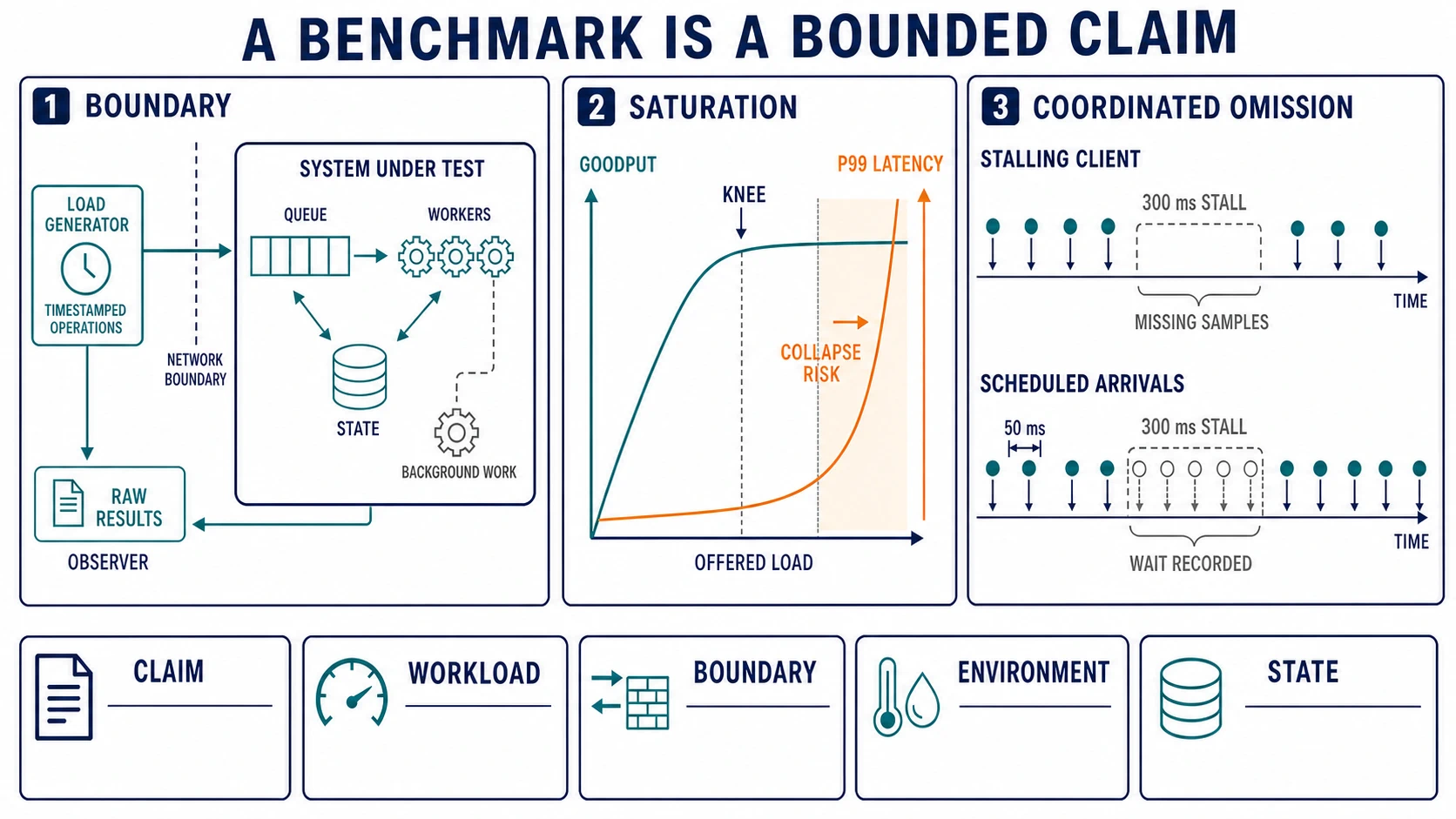
Calibrate the client independently. Establish its maximum scheduled rate using a cheap target or no-op protocol path, while retaining timestamp, serialization, network, response validation, and raw-record costs. Generator capacity should exceed the highest offered rate with explicit headroom. Monitor its CPU, run queue, socket errors, clock behavior, buffers, and dropped measurements during the real test.
Multiple generators can add capacity but introduce clock, coordination, and aggregation problems. Prefer client-side elapsed time from a monotonic clock for each operation. If server and client timelines must be joined, measure synchronization error and do not subtract timestamps across hosts as though their clocks were exact.
Record offered, admitted, started, completed, correct, failed, timed out, cancelled, and retried counts. Conservation checks catch missing work:
offered = rejected before admission + admitted
admitted = queued/in flight at end + terminal outcomes
logical operations ≠ attempts when retries occur
If counts do not reconcile within a declared loss policy, do not publish latency percentiles from the surviving subset as if it were the workload.
Open and closed generators ask different questions
A closed workload maintains a fixed client population. Each client often waits for completion, optionally thinks, then submits again. When the server slows, the clients naturally send less work. This is representative of some interactive sessions and fixed worker populations. It is not representative of exogenous arrivals that continue while service degrades.
An open workload schedules arrivals independently of prior completions. It can expose queue growth and overload under a fixed offered-rate process. If the harness cannot maintain the schedule, it must record lateness or missed arrivals rather than shifting their timestamps forward and claiming the intended rate.
Neither model is universally correct. Select the model from production demand. A mobile user may behave partly closed; a broker backlog or scheduled event stream behaves more openly; retries add feedback. State think-time distribution, client concurrency, connection reuse, timeout, retry, and abandonment behavior as workload inputs.
Coordinated omission removes the moments you needed to measure
Coordinated omission occurs when measurement timing depends on the system’s ability to respond. A client submits one request, waits through a stall, then resumes. It records one long latency while omitting the requests that would have arrived during the stall. The measured population becomes sparse precisely when service is worst.
The fixture models 10,000 ordinary 8 ms observations and thirty 300 ms stalls. A closed client records one 300 ms observation per stall: 10,030 observations total, with p99 still 8 ms. Scheduled arrivals every 50 ms represent six affected observations per stall—300, 250, 200, 150, 100, and 50 ms—giving 10,180 observations and p99 150 ms.
This is a simulated population demonstration, not a general post-processing recipe. Correct repair is to generate or reconstruct the intended arrival schedule, timestamp before send, retain lateness, and define what happens when the client cannot keep up. Histogram correction from an expected interval can be useful when its assumptions hold, but it cannot recover an unknown production arrival process or missing correctness outcomes.
Ask three questions of every latency report:
- What caused each observation to be scheduled?
- Which intended observations could not occur or were discarded?
- Does latency begin at intended arrival, actual send, admission, service start, or another boundary?
A low p99 with a stalling generator may be an accurate percentile of the wrong population.
Sweep offered load through the knee
A single “maximum throughput” number hides the operating curve. Hold workload and state constant, increase offered load in deliberate steps, and record goodput, latency distribution, queue age, resource demand, errors, and client health. Use ramp periods only to reach state; retain independent holds long enough to observe variability and background cycles.
The simulated Mercury subsystem uses an external generator calibrated to 4,000 operations/s and never offers more than 1,800/s, a 2.22× rate headroom. Five independent runs at each point produce these means:
| Offered/s | Mean goodput/s | Mean p99 |
|---|---|---|
| 400 | 397.8 | 34.0 ms |
| 800 | 795.0 | 38.0 ms |
| 1,200 | 1,178.0 | 51.4 ms |
| 1,400 | 1,325.0 | 78.0 ms |
| 1,600 | 1,360.0 | 189.8 ms |
| 1,800 | 1,300.0 | 620.0 ms |
The knee lies between 1,400 and 1,600 offered/s for the declared objective: goodput gains only 35/s while p99 more than doubles and completion efficiency falls below 90%. At 1,800/s, goodput decreases while latency explodes. The useful result is not “capacity is 1,360/s.” It is the curve, operating criterion, environment, and uncertainty around the transition.
Saturation tests need abort criteria. Stop when queue age threatens data retention, correctness errors appear, the generator loses schedule, telemetry buffers overflow, or recovery would exceed the test’s blast radius. After each high-load point, verify the system returns to its declared state. Carrying backlog or hot caches into the next run makes load order part of the treatment.
Repetition reveals variance; it does not manufacture independence
One run cannot characterize run-to-run variability. Repeat complete experimental units, preserving raw observations and per-run summaries. Report the number of independent runs, within-run population, central effect, dispersion or interval, and practical threshold. Do not pool millions of request observations from one host and call them millions of independent experiments.
Sample size should follow the decision and noise structure, not a ritual minimum. High percentiles require enough representative observations in the target population; rare failure states may require designed scenarios rather than longer nominal runs. A small effect below run-to-run noise needs better control, pairing, more independent runs, or rejection as operationally irrelevant.
Effect size is the change with units or a meaningful ratio. “Statistically significant” does not answer whether a 0.3% CPU change justifies complexity. Conversely, a 10% tail improvement may be inconclusive if workload drift is 15%. Chapter 53 supplies confidence intervals, blocking, randomization, sequential-test warnings, and distribution comparisons. Here, the benchmark must retain the raw experimental units those methods require.
Do not average host p99 values and present the result as a fleet p99. Merge compatible distributions or raw histograms with their counts and definitions, or report host-level variation separately. Percentiles depend on a population; averaging them changes that population without a clear quantile meaning.
Microbenchmarks have special failure modes
A microbenchmark can accidentally measure everything except its claim:
- the compiler eliminates unused work or folds a constant result;
- setup, allocation, or teardown enters or leaves the timed region inconsistently;
- timer overhead is comparable to the operation;
- one repeated input creates unrealistic branch and cache state;
- batched iterations hide per-operation tail or cancellation behavior;
- a CPU frequency, thermal state, or competing process changes across variants;
- manual timing records asynchronous launch but not completion;
- correctness validation is absent, so a broken fast implementation wins.
Prevent elimination by consuming outputs through a mechanism the compiler cannot prove irrelevant, but do not let that mechanism dominate the timing. Calibrate the empty loop and timer. Vary inputs according to the claim. Separate CPU time from elapsed time when waiting or asynchronous devices matter. Store compiler, flags, binary digest, runtime, host topology, and power policy.
The fixture’s encoder claim explicitly includes the function, buffers, digest, 8 KiB size, fixed entropy distribution, warm process, and one calling thread. It excludes the network, outer allocation, queueing, multi-core scaling, cold start, and production mix. If Chapter 50 shows encoding is 2% of the endpoint’s CPU and CPU is not the constraint, even a 50% microbenchmark win predicts at most a small local effect and may not deserve integration.
Honest mistakes can look like benchmark fraud
Misleading reports often arise without intent:
| Practice | Why it biases the claim | Repair |
|---|---|---|
| best run or best window | selects favorable noise/state | predeclare inclusion; publish every valid run |
| mismatched durability | variants acknowledge different effects | define correctness and commit boundary |
| failed requests removed | rewards overload or broken output | report all outcomes; count correct goodput |
| candidate-only tuning | compares methods and environments together | apply symmetric policy or declare treatment |
| one payload or key | hides distribution and skew | trace production-relevant dimensions |
| server timer only | omits queues/network/client wait | align boundary with claim |
| benchmark after manual cleanup | removes ordinary background cost | include or explicitly scope state |
| generator at 100% | client limits offered load and timestamps | calibrate and monitor with headroom |
Named benchmark suites add formal run and reporting rules precisely because comparability requires more than code. Do not borrow a suite’s metric name, alter its workload, and imply comparison with conforming results. A derived workload is a new claim with its own disclosure.
The manifest is part of the result
A reproducible result retains enough custody to rerun and audit the experiment:
| Manifest group | Required contents |
|---|---|
| decision | claim, owner, hypothesis, acceptance/rejection rule |
| boundary | topology, clocks, timed region, unit of work, correctness |
| workload | arrival model, mix, distributions, data generator/digest, client behavior |
| environment | hardware/topology, quotas, OS/runtime/build, flags, configuration |
| state | preparation, warm-up rule, background work, reset, run order |
| execution | commands, seeds, repetitions, duration, aborts, generator calibration |
| evidence | raw observations/histograms, logs, errors, hashes, missingness |
| analysis | scripts/version, exclusions, uncertainty, figures, result tables |
| validity | confounders, deviations, transfer limits, unresolved questions |
Use immutable identifiers or hashes for code, configuration, data, and raw artifacts. Store a human-readable report beside machine-readable inputs. A chart without raw counts and a manifest is a presentation, not evidence custody.
Run the retained teaching packet:
node examples/performance-engineering-system-design-handbook/part-06/benchmark-validity/run.mjs
node examples/performance-engineering-system-design-handbook/part-06/benchmark-validity/verify.mjs
Then audit four claims. First, repair the 31% opening result by writing its five nouns and a symmetric state rule. Second, explain why the closed generator’s p99 stays at 8 ms and name the production arrival assumption needed for scheduled repair. Third, review a storage comparison in which one variant acknowledges a memory buffer and the other flushes durable bytes; decide whether to align durability or narrow the claim. Fourth, write a microbenchmark transfer statement that names one represented distribution, two excluded system costs, and the profile evidence required before architecture changes.
A final review can be short: Is the unit correct useful work? Does the workload preserve causal production dimensions? Are generator, clocks, and missing arrivals visible? Is the intended state reached and ordinary background work represented? Are variants treated symmetrically? Do repeated raw runs support an operationally meaningful effect? Can another engineer reproduce the environment and analysis? Does the claim stop exactly where the evidence stops?
A benchmark result is valid only for the claim, workload, boundary, environment, and state represented by the experiment. Publish all five with raw custody and transfer limits. Chapter 52 expands the experiment from a steady saturation curve into load, spike, soak, failure, and recovery phases; a benchmark that cannot preserve its contract across those phases must not be used to predict them.
Sources and evidence scope
- Google Benchmark user guide documents warm-up time, independent repetitions, raw JSON/CSV output, counters, manual timing, random interleaving, and variance-reduction controls for a microbenchmark library. These features do not establish workload representativeness by themselves.
- HdrHistogram coordinated-omission guidance documents correction when an expected interval is known; the chapter treats that as conditional reconstruction, not a substitute for an independently scheduled generator.
- wrk2 methodology and implementation provides a constant-throughput generator designed to record latency without coordinating offered rate to response. Tool use still requires client calibration and a representative workload.
- SPEC CPU 2026 run and reporting rules illustrate how a benchmark suite controls builds, continuous execution, validation, configuration, and disclosure to preserve comparability.
- TPC fair-use quick reference distinguishes conforming published results from derived workloads and requires disclosure for the latter.
- All Mercury saturation, omission, generator, and microbenchmark values are simulated teaching evidence in
examples/performance-engineering-system-design-handbook/part-06/benchmark-validity/, not production observations or results from a named benchmark suite.