Performance Engineering and System Design Handbook / Chapter 4
Quantities, Units, and the Laws That Pay Rent
Use dimensional discipline and a small set of bounded models to reject impossible designs and choose the next decisive measurement.
Preparing audio…
Audio edition
Quantities, Units, and the Laws That Pay Rent
Write the unit beside the number before trusting the number.
That small habit catches a surprising class of architecture errors. A capacity sheet multiplies requests/s by ms and calls the result “threads,” while forgetting to divide milliseconds by 1,000. A network plan compares gigabits with gigabytes. A cache estimate counts payload bytes but omits indexes, allocator overhead, replicas, and the recovery copy. A parallelization proposal reports an eight-core speedup without naming whether the workload stayed fixed. None of these errors requires advanced mathematics. They require quantities that retain their meaning while they move through a model.
This chapter is a compact quantitative workbench. Its primary decision is: which cheapest model can disqualify a bad option, bound the value of an optimization, or identify the next measurement? The models pay rent only when their boundary and conditions survive contact with the system. They are filters for engineering judgment, not equations that manufacture evidence.
A quantity is a value with a meaning
A count answers how many units exist in a stated population: 180 accepted requests in the system. A rate divides a count by time: 2,400 completed requests per second. A duration is time per event: 75 milliseconds per completed request. A ratio divides like quantities and is dimensionless, although its population still matters: 2.5 network bytes per logical byte. A work-normalized metric divides resource consumption by useful outcomes: 3.2 CPU milliseconds per correct search response, not per attempt.
The label is part of the datum. 2,400 requests/s is incomplete if “request” mixes cheap cache hits, wide searches, retries, and rejected attempts. Chapters 2 and 3 supplied the workload population and desired outcome; this chapter insists that every calculation preserve them.
Dimensional analysis asks whether the units on both sides of an equation agree. If completion rate is requests/s and mean residence time is s/request, their product is requests. If the sheet produces requests²/s, the operation is wrong regardless of how plausible the number looks. Unit agreement does not prove a model is applicable, but disagreement proves it is not.
Magnitude and conversion reference card
| Quantity | Safe expression | Conversion or warning |
|---|---|---|
| time | ns, µs, ms, s | 1 s = 1,000 ms; convert before multiplying by /s |
| decimal data | kB, MB, GB | powers of 1,000; common for line rates and vendor storage |
| binary data | KiB, MiB, GiB | powers of 1,024; do not silently relabel as decimal |
| bits and bytes | bit, B | 8 bit = 1 B; 10 Gbit/s is not 10 GB/s |
| event rate | events/s | name offered, accepted, completed, or useful events |
| bandwidth | bit/s or B/s | state payload versus protocol/on-wire bytes |
| utilization | busy time / available time | a ratio over a named resource and interval, not “load” |
| service demand | resource time / completed unit | differs from elapsed response time when waiting or parallelism exists |
| throughput efficiency | useful units / resource | name correctness and success criteria |
| amplification | physical work / logical work | numerator and denominator must use the same base dimension |
Scientific notation keeps magnitude visible: 4 × 10^8 bit, not an ungrouped string of zeros. Carry more precision during a calculation than the inputs justify only to avoid intermediate rounding; report the result as a range or rounded magnitude. An estimate from 60–90 ms and 1,800–2,600 requests/s should not end as 171.36 concurrent requests.
Reconstruct concurrency with Little’s Law
Mercury’s gateway completed an observed mean of 2,400 accepted search requests per second during a stable ten-minute interval. The same population spent an observed mean 75 milliseconds from gateway admission through final response. The concurrency gauge is missing. With L as mean units in the bounded system, λ as mean completion rate, and W as mean time in that system:
L = λW
  = (2,400 requests/s) × (0.075 s/request)
  = 180 requests
The reconstructed mean is 180 in-flight accepted searches. It is not a p99 concurrency, a thread count, or a recommended pool size. It includes whatever the chosen residence boundary includes—service, queue, dependency waits, and response work—and it excludes work outside gateway admission or after final response.
Little’s Law is broad, but it is not boundary-free. Use the same population for L, λ, and W; measure over a sufficiently stable interval; account for abandonment or use the appropriate effective rate; and interpret the result as a long-run mean. During an accumulating backlog, arrivals can exceed departures while the population rises, so multiplying a short-window departure rate by latency can conceal the transient. During recovery, old backlog and new traffic may be different populations.
The law is useful in both directions. If a service reports 900 mean in-flight units and 2,400 completions/s at the same boundary, the implied mean residence time is 900 / 2,400 = 0.375 s. If the latency dashboard says 75 ms, the disagreement is a diagnostic gift: boundaries, populations, averaging windows, or instrumentation differ. Do not “fix” the sheet until the team explains the discrepancy.
For uncertain planning inputs, retain the rectangle rather than multiplying midpoints. Mercury’s estimated arrival envelope of 1,800–2,600 requests/s and residence range of 60–90 ms implies a coarse concurrency range from 1,800 × 0.060 = 108 to 2,600 × 0.090 = 234. That conservative cross-product assumes the high values may coincide. If telemetry establishes a joint relationship, replace the rectangle with that evidence.
Bound parallel work before building it
Amdahl’s Law addresses fixed work. Let s be the fraction of elapsed work that remains serial and N the parallel capacity. The ideal speedup is:
S_fixed(N) = 1 / (s + (1 - s) / N)
If profile evidence attributes 25% of a fixed job to an unavoidable serial stage, eight ideal workers offer at most:
1 / (0.25 + 0.75 / 8) ≈ 2.91×
Even infinite parallel capacity approaches only 1 / 0.25 = 4×. If a proposed refactor costs three months and requires 6× speedup, the estimate has already rejected the current mechanism. Measure or redesign the serial portion before optimizing worker scheduling.
The bound is optimistic. It omits task creation, communication, load imbalance, memory bandwidth, synchronization, and tail effects unless those costs are included in s or modeled separately. “Serial fraction” is also workload- and scale-dependent. A lock, coordinator, or memory channel may become more expensive as workers grow.
Gustafson’s Law asks a different question: if available parallel capacity lets the problem grow while elapsed time stays roughly fixed, how much scaled work can be completed? With serial fraction s measured in the scaled execution:
S_scaled(N) = N - s(N - 1)
For s = 0.25 and N = 8, scaled speedup is 8 - 0.25 × 7 = 6.25×. This does not refute the fixed-work bound. One model says a fixed report will not become six times faster; the other says a larger report may process about 6.25 times the original work in the same elapsed budget, under its assumptions. A design review must name which claim the product needs.
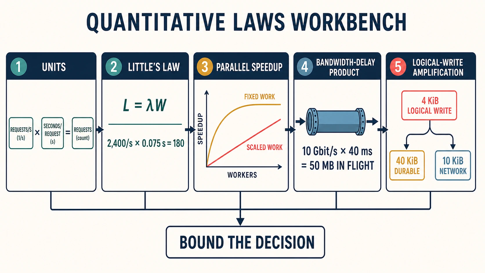
Speedup is a curve, not a core count
Workers N |
Amdahl, s=0.25, fixed work |
Gustafson, s=0.25, scaled work |
|---|---|---|
| 1 | 1.00× | 1.00× |
| 2 | 1.60× | 1.75× |
| 4 | 2.29× | 3.25× |
| 8 | 2.91× | 6.25× |
| 16 | 3.37× | 12.25× |
| infinity | 4.00× | not a finite fixed-work comparison |
The table is an illustrative model, not a benchmark. Its job is to expose the fixed-versus-scaled choice and the upper bound. Measure useful outcomes and correctness as workers rise. A 3× attempt-rate increase that produces duplicates, timeouts, or wrong results is not speedup.
Fill the path before blaming the endpoint
Bandwidth-delay product (BDP) is the amount of data that can be in flight when a path transmits at bandwidth B over round-trip time R:
BDP = B × R
    = (10 × 10^9 bit/s) × (0.040 s)
    = 4 × 10^8 bit
    = 50 MB
On this modeled 10 Gbit/s, 40 ms round-trip path, roughly 50 decimal megabytes must be in flight to sustain the nominal line rate. This is not a command to set one 50 MB socket buffer. Protocol windows, congestion control, loss, competing traffic, send/receive buffers, application concurrency, framing, and endpoint limits all affect realized goodput. The model says something narrower and valuable: a transfer design that permits only 4 MB outstanding cannot fill this path, even with zero server compute cost.
Keep payload goodput separate from wire rate. Headers, encryption framing, acknowledgments, retransmissions, and application amplification consume capacity. One-way latency cannot silently replace round-trip time in a feedback-limited calculation. In a multi-path system, one fleet-average RTT produces no real path; segment by route and state.
Resources per useful unit
Utilization is busy resource time divided by available resource time for a named resource and interval. At 70% CPU utilization, the remaining 30% is not interchangeable capacity for memory bandwidth, disk IOPS, network packets, locks, or a single hot core. Fleet CPU can be 35% while one serialization thread is saturated.
Service demand normalizes a resource by completions: CPU seconds per useful request, bytes read per query, storage operations per committed transaction. If throughput is X useful units/s and a resource provides C resource-units/s at the measured state, a first capacity bound is C / demand_per_unit. Use the bottleneck resource, not the most convenient fleet percentage.
Operational intensity relates computation to data movement:
operational intensity = operations / bytes moved
                      = 12 × 10^9 operations / 6 × 10^9 B
                      = 2 operations/B
The illustrative kernel performs two counted operations per byte moved at the measured boundary. That does not label it universally compute- or bandwidth-bound. Compare it with the applicable machine’s measured ceilings and include the bytes actually moved through the relevant memory hierarchy. An algorithmic operation count, cache-line traffic, and DRAM traffic are different boundaries.
Working set is a residency claim
A data set is everything retained; a working set is the data and metadata that must remain accessible with the intended locality over a relevant interval. Mercury has 8 million active records, each with a 240 B payload and 72 B of index material. An estimated allocator-and-metadata factor is 1.18:
bytes per replica
  = 8,000,000 records × (240 + 72) B/record × 1.18
  = 2,945,280,000 B ≈ 2.95 GB

two replicas ≈ 5.89 GB
This is a footprint estimate, not a promise that a 6 GB cache suffices. Object layout, alignment, fragmentation, auxiliary indexes, code, connection state, temporary results, kernel pages, eviction policy, and growth need explicit treatment. Replication may improve read capacity while multiplying memory and recovery traffic. During rollout or rebuild, old and new copies may overlap.
Test the cliff, not only the midpoint. If the active set ranges from 7–11 million records and metadata factor from 1.12–1.28, compute corners and ask when the working set no longer fits the intended tier. A design whose latency objective depends on 95% residency needs an eviction and warm-up experiment, not only byte arithmetic.
Amplification: where one logical operation multiplies
For one illustrative 4 KiB logical write, the fixture accounts for:
| Layer | Physical work | Relative to 4 KiB logical write |
|---|---|---|
| primary WAL | 4 KiB durable bytes | 1× |
| primary data/page work | 8 KiB durable bytes | 2× |
| replication payload | 8 KiB network bytes | 2× |
| replica WAL and data | 24 KiB durable bytes | 6× |
| expected background maintenance | 4 KiB durable bytes | 1× |
| expected retry traffic | 2 KiB network bytes | 0.5× |
| total durable | 40 KiB | 10× |
| total network | 10 KiB | 2.5× |
The stack deliberately keeps dimensions separate. Adding durable bytes and network bytes into “12.5× I/O” would erase which resource is constrained. Real systems also amplify reads, space, compaction, checksums, indexes, snapshots, and repair. A retry can multiply logical attempts without multiplying useful commits, so use request lineage and idempotency semantics when counting it.
Amplification can move rather than disappear. Batching may reduce per-write protocol overhead while increasing wait time and recovery burst size. Compression can reduce network and storage bytes while increasing CPU demand and tail variance. An index can reduce read amplification while increasing write and space amplification. Record numerator, denominator, operating state, and correctness boundary for every factor.
Fit scalability; do not worship the fit
The Universal Scalability Law (USL) is an empirical capacity model for normalized throughput or capacity C(N) at concurrency N:
C(N) = N / [1 + α(N - 1) + βN(N - 1)]
The parameter α captures a contention-like linear penalty in this model; β captures a coherency or coordination-like quadratic penalty. With illustrative α = 0.03 and β = 0.002, capacity rises, flattens, and eventually falls. The curve can expose a concurrency region where adding workers reduces useful throughput.
Do not assign causal mechanisms from fitted letters alone. Several real effects can produce similar curves: a lock, hot partition, memory bandwidth, cache coherence, downstream pool, retry feedback, or measurement distortion. Fit only comparable steady-state points with correctness held constant; inspect residuals and uncertainty; then use profiles, queue telemetry, traces, and controlled interventions to find the mechanism. Extrapolation beyond measured concurrency is a hypothesis.
USL differs from the preceding parallel laws. Amdahl bounds ideal fixed-work speedup from a serial fraction. Gustafson describes scaled work. USL fits observed capacity degradation as concurrency changes. Choosing one because it produces the preferred forecast is model shopping.
Estimate in ranges, then buy information
A back-of-the-envelope estimate should expose its input ledger:
| Input | Range | Evidence | Reversal risk |
|---|---|---|---|
| accepted arrival rate | 1,800–2,600 requests/s | observed recent windows | launch mix may exceed range |
| mean residence | 60–90 ms | observed nominal state | degraded dependencies change it |
| active records | 7–11 million | modeled growth range | migration timing uncertain |
| bytes/record before overhead | 280–340 B | measured sample and schema | variable fields have a tail |
| metadata factor | 1.12–1.28 | estimated | allocator/version dependent |
Multiply bounds when the quantities may coincide; use joint evidence when available. State whether a number is observed, estimated, modeled, simulated, or inferred. Round to the precision that can affect the decision. Then perform sensitivity analysis: which input range can reverse the choice between designs?
If both ends of a plausible retry factor keep network demand below 20% of capacity, refining it has low immediate decision value. If the working-set range straddles the memory tier, measure record footprint and locality next. The model has paid rent by directing evidence collection.
Field exercise: two decisions, not ten equations
Use model.json and the verifier. First reconstruct Mercury concurrency and explain why 180 is neither a pool recommendation nor a tail bound. Then choose one proposed optimization:
- parallelize the fixed report across eight workers;
- raise transfer concurrency on the 10 Gbit/s, 40 ms path;
- keep two active in-memory replicas after the next migration;
- batch logical writes to reduce amplification.
For the choice, state the useful unit, boundary, state, input ranges, model, and disqualifying threshold. Name one omitted mechanism that could reverse the conclusion and one measurement that would resolve it. For parallelism, distinguish fixed from scaled work. For networking, distinguish line rate from goodput. For memory, include working set, replicas, and overlap during recovery. For writes, keep durable, network, CPU, and latency dimensions separate.
Run the fixture:
$ node examples/performance-engineering-system-design-handbook/part-01/quantities-and-tails/verify.mjs
quantities: verified Little=180, BDP=50 MB, USL points=7
tails: verified n=1000, mean=68.8675 ms, p99=680 ms, fan-out=33.1%
The program checks arithmetic and declared units encoded in the fixture. It cannot prove stable means, representative traffic, causal parameters, or achievable hardware performance.
Decision rules
- Attach a population, boundary, interval, operating state, and unit to every consequential number.
- Reject equations whose dimensions do not balance before debating their inputs.
- Use Little’s Law to reconcile long-run mean population, effective rate, and residence time only at matching boundaries.
- Use Amdahl for fixed work and Gustafson for scaled work; include coordination and correctness costs before making a speedup claim.
- Use bandwidth-delay product to bound required in-flight data, not to promise transport goodput.
- Normalize resources by correct useful work, and keep different physical resources out of one amplification total.
- Treat USL parameters as empirical curve terms that guide diagnosis, not automatic root-cause labels.
- Prefer a range that preserves uncertainty over precision unsupported by inputs; measure next where uncertainty can reverse the decision.
These models mostly operate on means, bounds, and fitted capacity. They can reject impossible arithmetic while still missing the experience of rare work. The next question changes the object of analysis from one representative number to the entire distribution.
Sources and evidence scope
- NIST Guide to the SI, Chapter 7 supports the distinction between a quantity, its numerical value, its unit, and its dimension. SI conventions do not define application boundaries or useful work.
- Little, “A Proof for the Queuing Formula” establishes
L = λWunder stated long-run conditions. This chapter’s short operational checks require matching populations and stable-enough observation windows; the formula alone does not establish them. - Amdahl, “Validity of the Single Processor Approach” is the primary fixed-work speedup source. The 25% serial example is illustrative, not observed hardware evidence.
- Gustafson, “Reevaluating Amdahl’s Law” motivates scaled-work reasoning. It answers a different workload question from fixed-work speedup.
- RFC 6349, Framework for TCP Throughput Testing defines BDP in a TCP throughput-testing context. The 10 Gbit/s path is modeled and omits protocol and endpoint limitations.
- Gunther, “A General Theory of Computational Scalability Based on Rational Functions” develops the rational scalability model used here. Fitted parameters and extrapolated capacity need empirical validation and do not identify a mechanism by themselves.
- All Mercury quantities and fixture outputs are illustrative. The dependency-free verifier establishes internal arithmetic only.