Performance Engineering and System Design Handbook / Chapter 5
Distributions, Variance, and Tail Behavior
Read complete latency populations, quantify tail amplification, and compare distributions without letting averages or unscoped percentiles erase risk.
Preparing audio…
Audio edition
Distributions, Variance, and Tail Behavior
Which of these systems is healthier?
- System A averages 70 ms and has p99 latency of 220 ms.
- System B averages 55 ms and has p99 latency of 680 ms.
- System C reports p99 of 140 ms for successful responses and omits 2% timeouts.
There is no defensible answer. The populations, intervals, workloads, outcomes, sample counts, and objectives are missing. System C may have the prettiest line and the worst user experience. System B may contain one legitimate slow request class that should have its own objective. System A’s “p99” may be an average of per-host p99s, which is not the fleet quantile at all.
Unit discipline makes a calculation coherent; population discipline makes its conclusion honest. The primary decision is: which representation and segmentation reveal the probability of violating a user or capacity objective, and which evidence can distinguish mechanism from measurement artifact? The work is practical: retain enough of the distribution to see mixture, variance, and rare paths; then resist claiming more certainty than the sample supports.
Latency rarely has one symmetric cause
Many latency and service-demand populations are non-negative, asymmetric, multimodal, and state-dependent. A request may hit or miss a cache, wait or not wait for a lock, take a local or remote path, trigger zero or many dependencies, use a small or large payload, or overlap a collection pause. Queues add a lower bound near service time and a potentially long right tail. Timeouts truncate observations. Retries create related attempts. A normal distribution is not the default simply because a dashboard offers mean and standard deviation.
The companion fixture contains an illustrative population of 1,000 successful Mercury search responses:
- 760 cache-hit observations grouped from 18–55 ms;
- 200 cache-miss observations grouped from 116–190 ms;
- 40 degraded-dependency observations grouped from 180–989.75 ms.
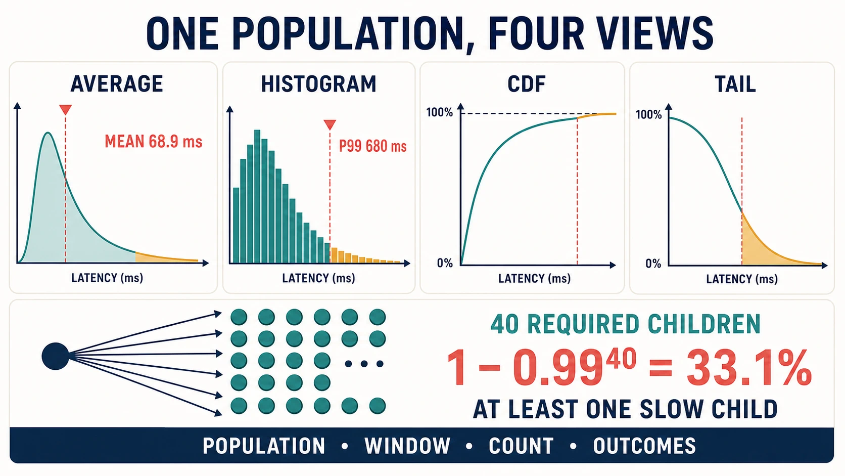
Its mean is 68.8675 ms, median 30 ms, p90 116 ms, p95 190 ms, and p99 680 ms under the declared nearest-rank definition. The mean lies above more than half the observations because a small slow population pulls it upward. Yet the mean alone does not reveal whether those observations are bad data, legitimate expensive work, or a failing dependency.
Four views answer four questions
Averages compress a population into its arithmetic center. They are useful for additive resource accounting—total CPU divided by completions, for example—but are weak descriptions of asymmetric latency.
A histogram groups observations into value intervals. It shows modes, gaps, and mass near an objective, but its resolution is limited by bucket boundaries. A p99 interpolated from a 500–1,000 ms bucket cannot justify a 20 ms distinction.
An empirical cumulative distribution function (ECDF) at value x is the observed fraction P(X ≤ x). It answers “what fraction completed within 250 ms?” and makes objectives readable as horizontal or vertical cuts. A quantile reverses that question: “what value is at or below a chosen fraction?”
A survival curve, P(X > x) = 1 - F(x), emphasizes the tail. A logarithmic probability axis can make rare exceedances visible without stretching the common case into a flat line. It must label zero handling and sample limits; with 1,000 observations, a supposed p99.99 has no empirical resolution.
A heat map adds time or another segmentation axis to distribution buckets. It can show a tail that appears only during deployment, a periodic job, a region incident, or tenant burst. It also prevents a long-window aggregate from blending a five-minute failure with hours of healthy service.
Define the percentile before debating it
For sorted observations x(1) ≤ ... ≤ x(n), this chapter’s fixture uses the nearest-rank definition: quantile q is x(ceil(qn)). Libraries use other exact or approximate definitions, especially interpolation between ranks. Two systems can legitimately produce slightly different p99 values from the same small sample. Record the estimator or telemetry type when that difference matters.
More important, a percentile is a property of a population:
p99 latency for successful and timed-out Mercury interactive searches, measured at the gateway from admission to terminal outcome, in
eu-westduring the 10:00–10:10 UTC launch window,n = 84,210, with timeouts represented at their observed terminal duration and outcomes reported separately.
That sentence states operation, class, boundary, geography, interval, state, count, and outcome treatment. “Fleet p99 = 180 ms” states almost none of them.
Quantiles do not compose by ordinary arithmetic. You cannot add a service’s p99 to a database p99 and call the sum end-to-end p99; the slow events may occur on different requests or may correlate strongly. Nor can you average host p99 values to obtain fleet p99. Aggregate raw observations, compatible histogram counts, or a mergeable distribution representation first, then calculate the target quantile over the intended population.
The fixture includes a four-request serial trace:
| Request | Stage A | Stage B | Joined total |
|---|---|---|---|
| 1 | 10 ms | 50 ms | 60 ms |
| 2 | 12 ms | 40 ms | 52 ms |
| 3 | 14 ms | 30 ms | 44 ms |
| 4 | 16 ms | 20 ms | 36 ms |
The stage values are anti-correlated. Summing component maxima produces 66 ms, although no request took 66 ms. With positive correlation the reverse risk appears: separate summaries can conceal that slow stages align on the same requests. Preserve request joins or directly measure the end-to-end boundary.
Coordinated omission manufactures a calm tail
Suppose an external production population attempts one request every 10 ms. The system pauses for one second. A closed-loop test client sends a request, waits for its response, then sends the next. During the pause it records one slow request and sends none of the requests that production would have attempted. Offered load falls exactly when service slows. The measurement coordinates sampling with system completion and omits the waiting opportunities.
Correction requires workload semantics, not a cosmetic percentile adjustment. Prefer an open arrival schedule when production arrivals are externally paced. Record intended send time, actual send time, admission, terminal outcome, and generator lag. If the generator misses scheduled arrivals, count and expose them. A post-recording correction such as HdrHistogram’s expected-interval methods can estimate omitted values under a declared schedule, but it cannot reconstruct arbitrary production behavior, request correlation, admission decisions, or failures.
Other distortions recur:
- success-only latency removes timeouts, cancellations, and malformed outcomes;
- client timing excludes DNS, connection setup, retries, or response consumption that the user sees;
- server timing includes queue admission only after an upstream queue;
- coarse buckets interpolate a quantile across a wide value interval;
- sampling drops rare slow traces disproportionately or without a known policy;
- clock error corrupts cross-host stage subtraction;
- warm-up, deployment, recovery, or cache-fill samples are blended into steady state;
- a timeout cap right-censors the true completion time and creates a spike at the deadline.
Do not “repair” a censored population by pretending every timeout equals its unknown natural duration. Report terminal user latency, timeout fraction, and separate censored analysis when needed. Correctness and outcome stay alongside latency.
Fan-out turns a small child tail into a common parent event
If a parent needs all n children and each child independently has probability p of exceeding a threshold, the probability that at least one child is slow is:
P(at least one slow) = 1 - (1 - p)^n
For 40 required children with independent 1% slow probability:
1 - 0.99^40 ≈ 0.331
About 33.1% of parent requests would encounter at least one slow child under this modeled independence assumption. The calculation is not the parent’s p99 latency. Parent behavior also depends on parallel launch, joins, cancellation, hedging, deadlines, partial-result policy, and how child delay translates to completion.
Independence is often false. A shared rack, region, shard, lock, network path, deployment, or garbage-collection trigger creates positive correlation; one event slows many children. Load balancing or diversified placement can create different dependence. Measure per-parent child outcomes and failure-domain labels. Sensitivity-test both independent and correlated cases when topology is uncertain.
Serial composition amplifies tails differently. Elapsed stages add for each joined request, but their quantiles do not. Queueing at one stage can change arrival burstiness at the next. Retries add serial or overlapping work and may select the same unhealthy dependency. The critical-path trace, not a spreadsheet of local percentiles, is the composition evidence.
Mixtures are often the mechanism
The fixture’s overall distribution is a mixture of cache hits, misses, and degraded dependency paths. Decomposition changes the engineering decision:
| Class | Count | Share | Range in fixture | Plausible next evidence |
|---|---|---|---|---|
| cache hit | 760 | 76% | 18–55 ms | hit validity, lookup and serialization cost |
| cache miss | 200 | 20% | 116–190 ms | backend path, payload/fan-out, queue time |
| degraded dependency | 40 | 4% | 180–989.75 ms | dependency outcome, retry lineage, failure domain |
An overall p99 of 680 ms does not mean the fastest 99% follow one mechanism. It cuts through the degraded mixture. Optimizing hit serialization by 5 ms may improve the median while barely moving p99. Improving dependency isolation may reduce the tail without changing the common path.
Segment by a hypothesis-bearing dimension: cache state, request type, tenant class, region, payload band, fan-out, code path, outcome, or deployment version. Avoid arbitrary high-cardinality slicing that creates noisy cells and privacy risk. Predeclare the primary cuts for an experiment; use exploratory cuts to form hypotheses that require confirmation on new data.
Simpson’s paradox can reverse an aggregate comparison. Imagine version B is faster than A for both cache hits and misses, but B receives a much larger share of misses. The fleet distribution can look slower despite within-class improvement. Conversely, a routing change that shifts easy traffic onto a canary can make a regression look like a win. Compare both standardized class distributions and the real production mix; they answer mechanism and user-impact questions respectively.
Variance consumes capacity and reliability margin
Two services can have identical mean service demand but different variance. The variable one produces more uneven completions, queue occupancy, connection holding, memory residency, deadline misses, and autoscaling signals. Near a constrained resource, bursts of long work let arrivals accumulate behind them. Queue analysis will derive the nonlinear behavior; the immediate rule is that mean demand alone cannot establish headroom.
Variance can come from useful diversity—large versus small queries—or from avoidable mechanisms such as lock convoying, noisy neighbors, retry storms, storage pauses, CPU migration, allocation, or shared dependency congestion. Removing legitimate expensive work may violate product semantics. Splitting it into a separate class, limiting fan-out, precomputing, scheduling fairly, or assigning a distinct objective may be the correct design.
Operational controls affect the distribution. Admission can reject excess work quickly, improving admitted latency while lowering acceptance. Bounded queues truncate waiting but create explicit overload outcomes. Hedging may reduce individual tails while increasing shared load. Larger batches can improve throughput and worsen wait variance. Every tail optimization must report offered, admitted, correct, timed-out, and rejected populations plus resource demand.
Recovery is a distinct distribution. Cache warming, backlog replay, replica catch-up, and repair compete with new work. A nominal dashboard that excludes recovery answers the wrong capacity question. Keep operating envelopes and outcome objectives attached to the distribution.
Outlier, rare event, or defect?
An outlier is a relationship to a model, not permission to delete a row. A 900 ms observation may be:
- a legitimate expensive query in scope;
- a rare but valid failure/recovery path;
- a timeout represented at its deadline;
- a clock jump, duplicate record, unit conversion error, or instrumentation bug;
- traffic from the wrong population;
- evidence that the assumed distribution family is wrong.
Investigate lineage before exclusion. Retain raw or reproducible identifiers under appropriate privacy controls, record the exclusion rule before comparing variants when possible, and publish results with and without disputed observations if the decision changes. Winsorizing or trimming can answer a deliberate robust-center question; it cannot establish user tail behavior.
Data-quality checks should include impossible negative durations, timestamps outside the window, unit mismatches, count reconciliation across pipeline stages, duplicate event IDs, timeout and cancellation handling, bucket monotonicity, sampling policy, and clock provenance. A sharp new mode at exactly 1,000 ms may be a deadline, not a natural latency cluster.
High percentiles have sparse evidence
With n observations, the expected tail count beyond p99 is about 0.01n. At n = 1,000, only about ten observations determine the top 1%; p99.9 is effectively one observation under nearest rank. Reporting p99.99 from that sample adds decimals, not information.
The sample count needed depends on the decision, event dependence, estimator, desired confidence, and acceptable error. Requests in the same incident or burst are correlated, so a million events do not necessarily provide a million independent trials. Report the number of events, number of windows or independent experimental units, and the sampling design.
Confidence intervals describe sampling uncertainty under assumptions; they do not correct bias, coordinated omission, changing traffic mix, or a wrong boundary. Bootstrap intervals can be useful for a quantile when resampling respects the experimental unit. Resampling individual requests across a time-correlated incident destroys that structure; use blocks or repeated runs when appropriate. For an SLO threshold, the exceedance proportion and a binomial interval may be more stable and decision-relevant than an extreme quantile estimate.
Repeated experiments should randomize or alternate variants when time trends matter, retain warm-up and steady-state rules, and compare matched workload populations. “B’s p99 is 8 ms lower” is weak if bucket resolution is 50 ms or uncertainty intervals overlap broadly.
Compare distributions, not trophy percentiles
A useful comparison begins with the claim. If the objective is 250 ms, compare the fraction of eligible outcomes within 250 ms, timeout/rejection/correctness rates, and confidence or repeated-window variability. If the suspected mechanism affects cache misses, compare class-conditioned distributions and class mix. If the change trades median for tail, display an ECDF difference or several predeclared quantiles rather than choosing the favorable one after the fact.
Use an evidence table:
| Dimension | Baseline | Candidate | Interpretation boundary |
|---|---|---|---|
| offered attempts | same scheduled trace | same scheduled trace | generator lag reported separately |
| correct goodput | value and interval | value and interval | correctness oracle unchanged |
| ≤250 ms fraction | estimate and uncertainty | estimate and uncertainty | eligible outcomes declared |
| timeouts/rejections | separate counts | separate counts | never omitted from impact |
| p50/p95/p99 | same estimator and buckets | same estimator and buckets | sample count and resolution shown |
| resource/unit | CPU, bytes, I/O per correct result | same | catches tail improvement by excess work |
| segments | cache, tenant, region, outcome | same plus mix | distinguishes mechanism from mix shift |
Do not require stochastic dominance for every useful change; real trade-offs exist. Make the trade explicit. A candidate might reduce p99 and deadline misses while adding 4% CPU per correct result. The objective and resource budgets determine whether that is acceptable.
Diagnose three misleading dashboards
The fixture names three defects. For each, write the corrected query or collection plan and the decision it changes.
- Host-percentile average: a panel averages precomputed host p99s. Replace it with an aggregate over raw observations or compatible histogram buckets, preserving the intended labels, then calculate the fleet quantile. Also inspect per-host distributions for skew; fleet aggregation must not erase a hot host.
- Success-only latency: a panel reports 120 ms p99 while dropping timeouts. Add all terminal outcomes to the journey population, report latency and outcome separately, and evaluate goodput within the objective. Do not invent natural completion times for censored work.
- Closed-loop incident test: 50 workers wait for responses, so offered rate collapses during slowdown. Use an externally scheduled arrival process if that matches production, record generator lag and missed sends, and compare admission/overload policy at equal offered populations.
For the fan-out exercise, reproduce 1 - 0.99^40 ≈ 33.1%. Then replace independence with two extreme thought experiments: all child slow events are perfectly correlated, and slow events are spread so no parent sees more than one. Explain why topology and per-parent joins are the decisive evidence.
Run the dependency-free fixture:
$ node examples/performance-engineering-system-design-handbook/part-01/quantities-and-tails/verify.mjs
quantities: verified Little=180, BDP=50 MB, USL points=7
tails: verified n=1000, mean=68.8675 ms, p99=680 ms, fan-out=33.1%
The grouped sample is intentionally small and synthetic. It teaches calculation and representation; it establishes no Mercury production claim.
Percentile-reporting checklist
Before a percentile enters a review, incident, or experiment report, require:
- operation and traffic class;
- start/end boundary and clock source;
- geography, tenant or other necessary segmentation;
- operating state and workload envelope;
- exact time window and sample count;
- eligible outcomes, plus timeout, rejection, cancellation, and correctness treatment;
- quantile definition or approximation and histogram resolution;
- aggregation method—never an average of host or window quantiles;
- sampling policy and coordinated-omission controls;
- uncertainty or repeated-window variability appropriate to the decision;
- raw-data or reproducible-query path, retention constraints, and transfer limit.
If the checklist makes a panel title long, put the compact scope in the title and the full contract in panel help or an evidence ledger. Do not remove the scope from the analysis.
Decision rules
- Never report a percentile without the population, boundary, interval, count, outcomes, state, segmentation, and estimator needed to interpret it.
- Aggregate observations or compatible distribution representations before computing a fleet quantile; never average quantiles.
- Measure end-to-end composition directly or from joined request paths; component quantiles do not add.
- Match generator arrival semantics to production and expose scheduled, actual, admitted, completed, and omitted work.
- Decompose mixtures by causal hypotheses while retaining the real mix for user impact.
- Treat variance and rare paths as capacity and reliability inputs, not removable noise.
- Investigate outlier lineage and data quality before exclusion; disclose when an exclusion changes the decision.
- Match percentile precision to sample size, dependence, bucket resolution, and uncertainty.
- Compare outcome rates, threshold compliance, resource cost, and distributions—not one trophy percentile.
The average is no longer allowed to stand in for the population, but distribution knowledge alone does not explain the nonlinear rise in waiting near saturation. The next step follows these arrivals and service demands into queues, utilization, and backpressure.
Sources and evidence scope
- Prometheus, “Histograms and summaries” documents aggregation properties, bucket error, and why averaging precomputed quantiles is invalid in that telemetry system. Its implementation guidance does not choose a workload population or objective.
- HdrHistogram Java API documents expected-interval methods for coordinated-omission correction. Such correction depends on a declared schedule and does not reconstruct arbitrary production arrivals or outcomes.
- Google SRE, “Addressing Cascading Failures” motivates attention to tail latency, retries, deadlines, and overload interactions. It does not supply universal fan-out independence or timeout values.
- The 1,000-observation mixture, 33.1% fan-out calculation, serial trace, and dashboards are illustrative fixtures. Their verifier establishes counts and arithmetic, not distributional fit, causal attribution, or production transfer.