Performance Engineering and System Design Handbook / Chapter 2
Workload Models: Describe the Demand Before the System
Build a production workload envelope that preserves the demand dimensions capable of changing design and benchmark conclusions.
Preparing audio…
Audio edition
Workload Models: Describe the Demand Before the System
A request count is not yet a workload. Ten thousand cache hits, ten thousand image uploads, and ten thousand searches that each contact twenty shards can share a dashboard number while imposing radically different compute, memory, storage, and network demand. Even requests with the same route can differ by tenant, payload, key temperature, authorization path, outcome, or recovery state.
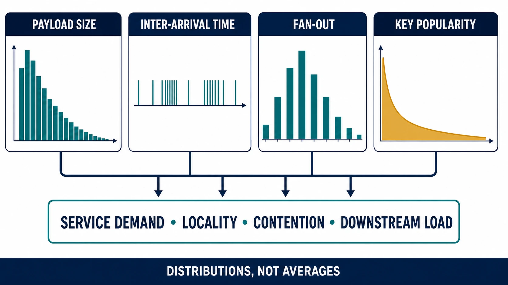
The useful abstraction is a distribution of units of work arriving under named conditions. Its job is not to reproduce every production detail. It must preserve every dimension capable of changing service demand, locality, contention, or downstream behavior. If omitting a dimension can reverse an architecture or benchmark conclusion, that dimension belongs in the model.
A performance contract already fixes a journey, boundary, useful outcome, and economic constraint. Keep those fixed here. The decision is narrower: what demand must the system satisfy, and which production properties must an experiment reproduce before its result can transfer?
Start with useful work, not endpoints
A unit of work should represent an outcome that can be counted consistently. “HTTP request” is often too coarse. For Mercury API, an interactive search outcome includes edge admission, authorization, retrieval, optional enrichment, and a correct response. An attempt that times out after issuing dependency calls consumes work but is not a useful outcome. Record both attempts and good outcomes.
Split a nominally identical operation when a characteristic materially changes cost or correctness. Candidate dimensions include operation and outcome, payload class, tenant class, geography, cache state, dependency path, priority, retry status, and cold/warm/recovering state. Do not split merely because a label exists; high-cardinality segmentation can make a model impossible to estimate. Merge classes only after evidence shows similar demand distributions.
The basic quantities answer different questions:
- Arrival rate, in units per second, describes how quickly new attempts appear.
- Concurrency, in in-flight units, describes how many overlap. It is affected by arrival rate and residence time, so it is not a synonym for traffic.
- Service demand, such as CPU-ms/outcome or storage bytes/write, describes resource work consumed, excluding or explicitly separating queue wait.
- Payload size and data-set size describe bytes per unit and total state. The same request distribution can behave differently when its working set no longer fits a cache.
- Completion rate counts finished attempts; goodput counts correct, useful outcomes. Retries and failures can increase completion activity while goodput falls.
Always attach units, population, interval, and state. “Peak traffic is 30” is unusable. “Observed 30 attempts/s for heavy-tenant interactive searches during this five-minute peak bucket” can be challenged and reproduced.
The workload-model canvas
Use one canvas per journey or materially different traffic class.
| Canvas field | Questions the model must answer |
|---|---|
| Boundary and useful unit | Which start/end events and correctness conditions define one outcome? |
| Intensity | What are arrival-rate and concurrency distributions by interval? |
| Mix | What fractions follow each operation, outcome, dependency, and read/write path? |
| Size and fan-out | What are payload, result, state touched, and dependency-count distributions? |
| Time | Is demand steady, bursty, periodic, diurnal, event-driven, or adversarial? |
| Skew and locality | Which tenants, keys, regions, and objects dominate; how quickly are they reused? |
| State | Which paths are warm, cold, degraded, rebuilding, or recovering? |
| Growth | Which drivers change smoothly, and which launches or migrations cause steps? |
| Evidence | Is each value observed, estimated, modeled, simulated, or assumed? From what interval? |
| Transfer limit | Which omitted or transformed property prevents a broader conclusion? |
The canvas is compact because its output is a decision input, not a telemetry inventory. Each row should point to evidence or an explicit assumption owner.
Open and closed demand are different experiments
In an open model, arrivals are scheduled independently of completion. If service slows, arrivals continue, concurrency and queueing can rise, and admission or overload behavior becomes visible. Public APIs, message ingestion, and timer-triggered work often need an open-model test.
In a closed model, a fixed population begins its next unit after completing the previous one, often after think time. When the system slows, that population generates fewer new units. Interactive sessions and fixed worker pools can legitimately be closed systems, but using a fixed number of load-generator workers to approximate an independent production arrival stream creates accidental feedback: the generator reduces offered load precisely when the system degrades.
OPEN                                    CLOSED
clock ──► arrivals ──► system           users ──► system
              │                            ▲         │
              └ independent                └ complete┘

slowdown: queue/concurrency can rise     slowdown: next arrivals are delayed
Neither model is universally superior. Match the causal source of demand. A system can contain both: customers arrive independently at an API, while each customer issues a dependent sequence of actions. Preserve both levels when session behavior changes cache reuse or request mix. Grafana k6’s current documentation distinguishes arrival-rate executors from virtual-user executors in this way; that is guidance about generator semantics, not proof that a chosen test matches production.
Mix multiplies into downstream work
Request mix is only the outer layer. Record the dependency mix and read/write ratio, because the same front-door rate can produce different internal demand. If Mercury’s heavy-tenant peak segment observes 30 attempts/s and p99 fan-out of 18, then a conservative tail-path estimate is:
30 attempts/s × 18 dependency calls/attempt = 540 dependency calls/s
This is estimated, not an observed simultaneous rate: multiplying marginal p99 fan-out by aggregate rate creates a stress-bound scenario, not a percentile of downstream traffic. The artifact retains the calculation because it is useful for disqualifying a dependency limit, while naming the transfer limit prevents it from masquerading as measurement.
Averages hide mixtures. Suppose searches are 80% two-shard lookups and 20% eighteen-shard lookups. The average fan-out is 5.2, but a generator that always issues five calls erases both the cheap locality and the expensive coordination path. Preserve categorical paths or draw from the empirical distribution; do not synthesize an “average request” that production never sends.
Four distributions, one workload
The outline’s example distribution set describes different causal levers:
| Distribution | Useful views | Mechanisms it can change | Common lossy substitute |
|---|---|---|---|
| Payload size | quantiles, tail exceedance, class-conditioned histogram | allocation, serialization, packets, storage I/O | one median-sized body |
| Inter-arrival time | gaps, bursts per short interval, autocorrelation | queueing, pool occupancy, scaling delay | constant requests/s |
| Fan-out | count by operation/outcome and required/optional branch | connection demand, tail amplification, dependency load | average dependency count |
| Key popularity | ranked share, top-k concentration, reuse distance | cache residency, lock/partition heat, replication | uniform random keys |
Do not assume these dimensions are independent. Heavy tenants may send larger payloads, choose wider searches, and concentrate keys during the same launch. Independent draws can create impossible combinations—small anonymous tenants with the heavy tenant’s privileged fan-out—or dilute the combinations that create overload. Preserve a joint table for the strongest correlations, then sample conditionally: tenant class first, operation within class, payload and fan-out conditioned on operation, keys from the class-specific popularity/reuse model.
Quantiles also answer different questions. A p99 payload describes a size threshold, not the identity of a p99-latency request. The largest payload may hit a local cache while a small request waits on a contended key. Joining per-request dimensions, under privacy controls, lets an experiment test mechanisms rather than multiplying unrelated percentiles. Where raw joins are prohibited, retain approved coarse classes and report the information loss as a transfer limit.
Time has shape
A daily average destroys the conditions under which queues and caches fail. Characterize demand at several useful intervals and name its source:
- steady baseline traffic tests sustained resource demand;
- bursts test queue bounds, admission, autoscaling delay, and connection limits;
- periodic jobs reveal synchronized work and shared-infrastructure coupling;
- diurnal traffic changes both intensity and often geography or mix;
- event-driven launches and incident retries introduce discontinuities;
- adversarial traffic concentrates expensive operations, keys, or invalid inputs.
Inter-arrival times show structure that a per-minute count cannot. Two five-minute windows can each contain 9,000 attempts. One may be nearly even; the other may contain six ten-second bursts separated by quiet gaps. The latter can exhaust pools even when average rate is identical. Retain a resolution fine enough for the shortest queue or resource tolerance relevant to the decision.
Skew is a resource map
Uniform traffic is a strong claim. Tenant concentration determines noisy-neighbor exposure. Hot keys concentrate locks, partitions, caches, and replication traffic. Heavy users may combine large payloads with high fan-out. Geographic imbalance changes network paths and failure domains. Popularity is sometimes usefully approximated by a Zipf-like curve, but the fitted family is secondary; measure the ranked shares and sensitivity rather than declaring a universal law.
State locality asks whether consecutive units reuse data, code, connections, or computed results. Cacheability asks whether reuse is legal and useful given freshness, authorization, and invalidation. Reuse distance counts distinct intervening references before an item is touched again; it predicts whether a finite cache may retain the item more directly than hit ratio alone. A shuffled trace can preserve key frequencies while destroying temporal locality, producing an invalid cache experiment.
A tenant-by-time heat map
The following compact table is an analytical heat map of illustrative offered attempts per five-minute bucket. It exposes concentration that a fleet total conceals.
| Bucket | Standard tenants | Heavy tenants | Heavy share |
|---|---|---|---|
| nominal | 18,000 | 2,000 | 10% |
| launch peak | 13,000 | 9,000 | 41% |
| dependency degraded | 6,000 | 4,500 | 43% |
| recovery replay | 5,000 | 12,000 | 71% |
These numbers are illustrative. The design implication is conditional: if heavy tenants also have larger payload and fan-out distributions, recovery capacity cannot be derived from fleet request totals. Test the joint segment, not each marginal dimension separately.
Model modes as envelopes, not one peak
A useful workload envelope names at least five operating modes:
- Nominal: expected mix with ordinary headroom.
- Peak: declared high demand with healthy dependencies.
- Degraded: one or more slow or unavailable dependencies, including retry policy.
- Recovery: backlog replay, cache warming, repair, or replica catch-up alongside new demand.
- Disaster: a bounded planning case such as region loss or data restore, with explicitly reduced objectives.
Peak and degraded are not interchangeable. Recovery can consume more storage and network work than peak user traffic. A disaster envelope is not “infinite load”; it is a chosen failure boundary and service policy.
Growth models need both slopes and steps. Organic demand might grow 4–7% per month, an estimated range. A tenant migration, product launch, retention-policy change, or new fan-out feature can add a discontinuity overnight. Record the driver, uncertainty, leading indicator, and date when a capacity or architecture decision must reopen. Extrapolating yesterday’s rate while payload and data-set size cross cache or partition thresholds creates a smooth forecast over a nonlinear system.
From telemetry to a reproducible model
The companion sample contains four Mercury segments. Run:
$ node examples/performance-engineering-system-design-handbook/part-01/workload-and-budgets/verify.mjs
workload model: verified 4 segments; peak p99 downstream demand 540 calls/s
budget worksheet: verified 250 ms allocation; observed burn 2.4x
For the workload exercise, inspect workload-sample.json. The validator checks that outcomes do not exceed attempts, p99 values do not fall below p50, required modes are declared, privacy fields exist, and the stated rate/fan-out arithmetic is consistent. It cannot prove representativeness or correlation.
Build a real model in four passes:
- Inventory: define the boundary, useful unit, traffic classes, modes, and candidate dimensions.
- Profile: compute counts and distributions at decision-relevant intervals; inspect joint segments rather than fleet aggregates alone.
- Challenge: ask which omitted dimension could reverse the pending choice. Compare the sample window with incident, launch, recovery, and seasonal windows.
- Package: retain queries or transformation code, an evidence timestamp, privacy treatment, raw-data location under access control, and a compact synthetic or de-identified fixture.
Trace replay preserves correlations and rare paths better than independent synthetic draws, but it can replay secrets, identifiers, pathological data, and outdated behavior. Remove unnecessary bodies, tokenize or bucket identifiers, enforce access and retention, and evaluate re-identification risk. NIST’s de-identification guidance explicitly warns that de-identified data can sometimes be re-identified; hashing a tenant ID is not automatically a privacy proof.
Synthetic generation is safer and controllable, but it must reproduce the decisive joint properties. Validate generator output against source distributions before using system results. Replay also requires time semantics: preserve or deliberately scale inter-arrival gaps, define how retries are handled, and decide whether state is warmed or reconstructed.
Construct the generator as a falsifiable artifact
A generator specification should be reviewable before it runs. For each generated field, record source evidence, transformation, correlation policy, random seed or replay cursor, and acceptance comparison. Then test the generator itself: do its five-minute burst counts, payload quantiles, segment mix, fan-out tail, top-key share, and reuse-distance bands match the intended envelope within declared tolerances?
Separate offered work from load-generation capacity. Instrument scheduler lag and dropped generation events. An open driver that cannot schedule its promised arrivals has silently become a lower-load test. Place generators so their CPU, network, connection, and address-space constraints do not become the system bottleneck; when distributed, verify clocks and aggregate the offered population without averaging node percentiles.
Correctness is part of workload generation. Provide an oracle for useful outcomes, stable request identifiers for detecting duplicates, bounded deadlines, and a rule for late completions. If production clients abandon work after a deadline, a replay that waits forever changes concurrency and resource reclamation. If production retries with jitter and a cap, unlimited immediate retries create a different workload. Model behavior, not merely messages.
Use sensitivity tests when evidence is uncertain. If top-key share is estimated between 20% and 35%, run both bounds and observe whether the decision changes. If both support the same cache or partition choice, additional precision may have low value. If the conclusion flips, collecting a better skew estimate is the next engineering task. Uncertainty becomes a test axis instead of a footnote.
Find the omission that invalidates the benchmark
Consider a benchmark that replays the correct operation ratio and fleet rate, uses production-sized median payloads, chooses keys uniformly, runs with twenty closed-loop workers, and reports average latency.
It fails four transfer tests:
- uniform keys erase the observed hot-key contention and locality;
- median payloads remove the heavy tail and its network/allocation cost;
- a closed generator reduces offered load during slowdown although production arrivals are independent;
- an average latency hides outcome and tail populations.
The most decisive omission depends on the claim. For a cache policy comparison, key popularity and reuse distance may invalidate it first. For admission behavior, the open/closed mismatch is fatal. For memory limits, payload tail may dominate. State the benchmark claim, then identify the omitted dimension that changes the causal mechanism behind that claim.
A counterexample is instructive: adding production skew can make a cache benchmark faster because hot objects fit, even while it makes a lock or partition benchmark worse. “Skew hurts performance” is not a rule. Skew changes locality and concentration; the mechanism decides the direction.
Field exercise: reconstruct demand from the sample
Using the fixture, produce a one-page canvas and answer:
- What is the useful unit and what work is counted only as an attempt?
- Which segment has the largest gap between offered rate and goodput?
- What design could be invalidated by ignoring tenant class?
- Which missing data—inter-arrival distribution, joint payload/fan-out observations, working-set size, or retry lineage—most limits a proposed overload test, and why?
- Design one open-model and one closed-model experiment. For each, state the production behavior it represents and the behavior it cannot establish.
- Add a disaster row without inventing an infinite peak: name the failure boundary, admitted traffic, reduced objective, and recovery interference.
Self-check the result. Every number must have a unit, population, interval, mode, evidence label, and transfer limit. Attempts and useful outcomes must remain distinct. At least one distribution must preserve a tail, and at least one joint segment must preserve correlation. The model should be small enough to drive a test, yet rich enough that removing any retained dimension would risk a different decision.
Decision rules
- Treat a benchmark as representative only when it preserves the production dimensions that materially affect service demand, locality, contention, and downstream behavior.
- Match generator feedback to the real arrival process; do not let a closed driver silently stand in for independent demand.
- Prefer named workload envelopes over one peak multiplier, especially for degraded and recovery states.
- Preserve joint segments when averages or independent sampling create units that production never sends.
- Collect the cheapest additional evidence that could reverse the decision; do not pursue a perfect model with no decision value.
The demand side is now explicit, but it still does not say what behavior is acceptable. The next decision assigns indicators and revisable budgets to these traffic classes and modes.
Sources and evidence scope
- Grafana k6: Open and closed models documents current generator semantics. It does not establish which model matches a particular production journey.
- NIST IR 8053: De-Identification of Personal Information supports the warning that de-identification reduces but does not eliminate re-identification risk.
- The Mercury sample and calculations are illustrative. The validator establishes structural and arithmetic consistency only; it provides no empirical performance result.