Performance Engineering and System Design Handbook / Chapter 62
Cost, Efficiency, and Sustainable Performance
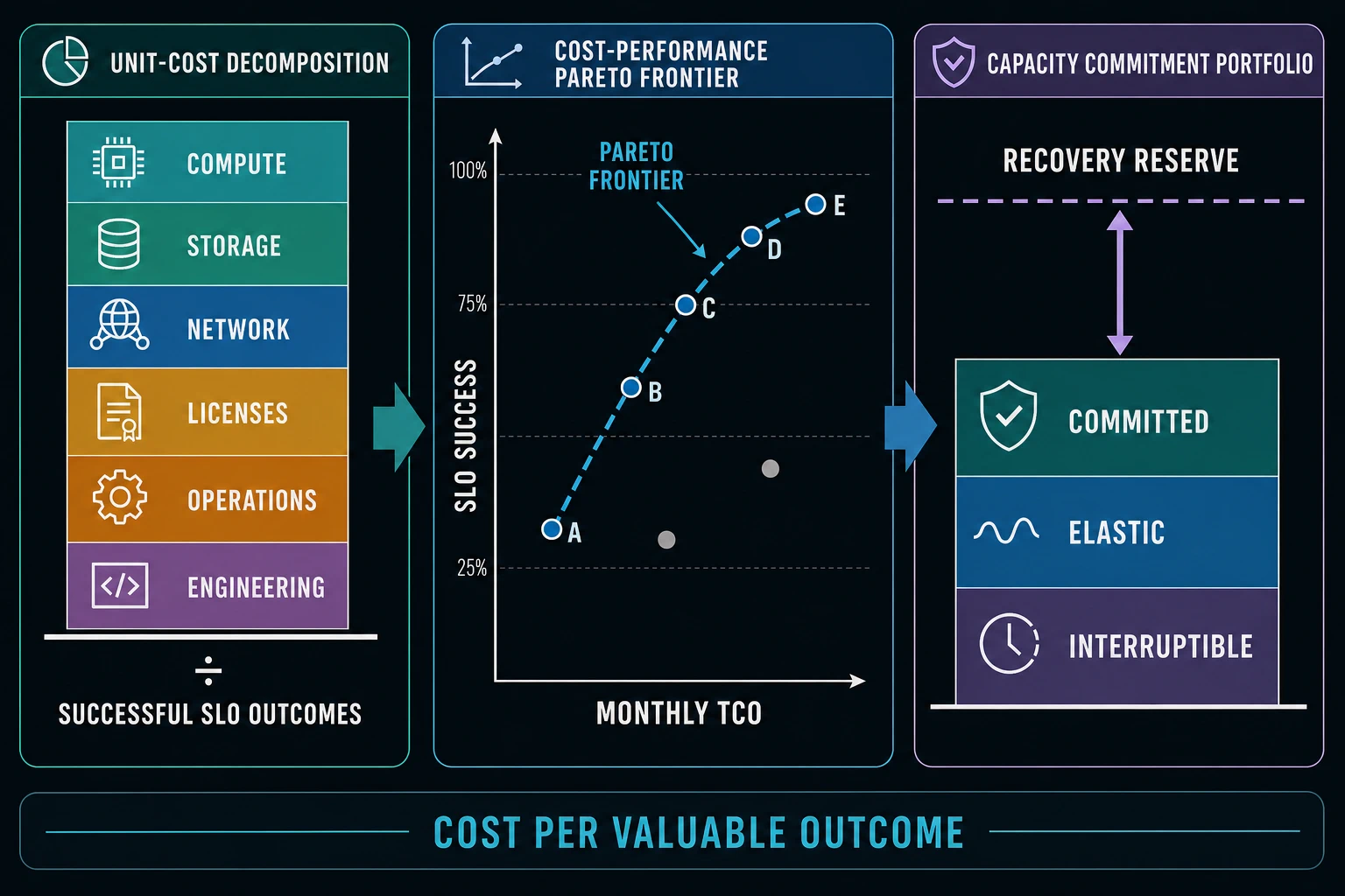
Compare designs by cost per valuable, correct, SLO-compliant outcome while accounting for headroom, labor, risk, data movement, energy, and rebound demand.
Preparing audio…
Audio edition
Cost, Efficiency, and Sustainable Performance
Two designs reach architecture review with one apparently decisive number:
| modeled month | lean shared design | isolated headroom design |
|---|---|---|
| compute + storage + network + licenses | $62,000 | $80,000 |
| fully loaded cost | $125,000 | $108,000 |
| correct SLO-compliant outcomes | 90.0 million | 98.5 million |
| cost per successful outcome | $0.001389 | $0.001096 |
The lean design wins an infrastructure-only comparison by $18,000. It loses after the ledger includes operations, engineering complexity, and reliability/recovery/compliance work. It also completes fewer valuable outcomes. The isolated design’s fully loaded cost is $17,000 lower and its cost per successful outcome is 21.06% lower.
This is not an argument that more infrastructure is always cheaper. It is an argument about the unit being optimized. Infrastructure spend is an input. A valuable, correct result inside its service objective is an outcome. The denominator must exclude attempts, failures, expired work, invalid outputs, and activity that does not create the declared value.
The decision rule is: optimize cost per valuable, correct, SLO-compliant outcome while accounting for risk, headroom, and operational labor. Absolute spend, utilization, energy, and unit cost remain necessary signals; none is sufficient alone.
Name the outcome before allocating cost
Choose a unit that follows the performance contract:
- a payment authorized once and durably recorded within its deadline;
- a search result returned within the freshness and relevance floor;
- a byte stored for the promised durability and retention period;
- a tenant query completed within its resource and isolation policy;
- a model output meeting the declared quality, safety, and latency bounds; or
- a business case resolved, not merely an API call emitted.
A resource-efficiency unit such as dollars per vCPU-hour, gigabyte, token, or request helps an engineer control a local driver. A business unit such as cost per successful checkout or cost per resolved case connects technology to value. Keep the mapping explicit. Reducing dollars per request while doubling requests per outcome is not an improvement.
For scope S and interval T:
UnitCost(S, T) = TCO(S, T) / N_valuable,correct,SLO(S, T)
Record population, workload mix, versions, region, service objective, correctness rule, allocation policy, shared-cost treatment, and uncertainty. The metric can otherwise improve because the team excluded hard tenants, loosened the SLO, stopped counting retries, or reassigned a shared platform bill.
Percentiles still matter. A monthly unit cost can conceal an expensive peak class or a tenant whose tail latency misses every objective. Slice by operation, tenant class, payload, region, hardware, cache state, failure mode, and deployment cohort far enough to expose causal drivers. Do not allocate so finely that measurement cost exceeds decision value.
The FinOps Foundation’s Unit Economics capability distinguishes resource-efficiency and business unit metrics and ties technology spend to organizational value. That supports the framing, not a universal denominator. Product and engineering owners must define what a valuable successful outcome means here.
Build a total-cost ledger that exposes transfers
Total cost of ownership includes costs that change because the design exists:
TCO = C_compute + C_storage + C_network + C_licenses
    + C_operations + C_engineering + C_risk
The categories need local definitions:
- Compute: steady and burst processors, accelerators, memory-coupled compute, orchestration overhead, and idle reserve.
- Storage: primary, replicas, indexes, snapshots, backups, logs, temporary spill, and deletion/retention work.
- Network: ingress where charged, cross-zone or cross-region transfer, egress, private connectivity, load balancing, and duplicated shadow traffic.
- Licenses and services: software, support, managed-service premiums, data/API access, and minimum commitments.
- Operations: on-call, incidents, capacity management, compliance evidence, migration, backup/restore tests, and vendor coordination.
- Engineering complexity: build, review, integration, performance validation, upgrades, debugging, and opportunity cost of specialist attention.
- Risk, reliability, recovery, and compliance: reserve, redundancy, insurance-like controls, failure exercises, reconciliation, and expected loss within the organization’s approved method.
Expected-loss estimates are decision models, not facts. Do not turn a low-probability catastrophic event into a precise-looking average without a scenario range and risk owner. Some compliance and correctness requirements are constraints, not costs to trade away. The ledger should reveal their resource consequence while preserving the obligation.
Use consistent time horizons. A one-time migration, three-year commitment, monthly bill, and weekly incident labor cannot be added without amortization and sensitivity. Separate cash spend from internal labor and opportunity cost so finance can reconcile money while engineering still sees displaced work.
The teaching comparison’s infrastructure categories total $62,000 and $80,000. Fully loaded categories bring the totals to $125,000 and $108,000. Those are modeled values, not provider prices. The reversal occurs because shared contention and weak isolation move expense into operations, engineering complexity, and recovery.
Classify cost behavior before forecasting it
Costs respond differently to demand:
- Fixed within a range: a control plane, minimum cluster, license floor, or on-call rotation exists even at low volume.
- Variable: bytes transferred, requests executed, accelerator-seconds, or object operations grow with units of demand.
- Step-function: another shard, replica set, availability cell, rack, license tier, or support team appears when a boundary is crossed.
- Mixed: a baseline commitment plus metered overflow combines all three.
Marginal cost asks what the next useful outcome costs before a boundary. Average cost spreads fixed and shared costs across all outcomes. Both are useful. A service can show falling average unit cost while approaching a step that makes the next tenant expensive. Capacity forecasts must mark those steps.
Allocate shared cost by the causal driver when possible: CPU-seconds, resident bytes, I/O, transfer, requests, retained history, support cases, or reserved capacity. Revenue share may be useful for budgeting but is not a performance cause. A tiny tenant with adversarial queries can create more cost than its revenue-weighted allocation reveals.
Track uncertainty as ranges. Demand, cache hit rate, compression, failure frequency, engineer time, and unit prices can all move. A useful model says which variable can reverse the decision. If a 3% change in cross-region bytes flips the architecture, instrument bytes and negotiate placement before claiming a durable choice.
Headroom purchases predictability
High utilization can reduce idle spend and increase queueing delay, tail variance, failure sensitivity, and recovery time. Headroom is not one undifferentiated buffer. Name what it buys:
- ordinary demand variance;
- forecast error and growth lead time;
- one tested failure domain;
- deployment and cold-start capacity;
- backlog drain and repair;
- tenant skew or hot partitions; and
- control and observation traffic during incidents.
Count the same reserve only once. A 20% buffer cannot simultaneously cover a 20% traffic spike, a cell loss, and a migration if those conditions can overlap. Model correlated scenarios and state which risks may share reserve.
Predictability has economic value even when the reserved resource looks idle. It can reduce deadline misses, incident labor, emergency purchases, customer credits, and the time engineers spend defending a fragile peak. That value still needs evidence. A fleet at 35% utilization with no documented failure envelope is not automatically prudent.
Queueing makes the trade-off nonlinear. As a constrained resource approaches saturation, a small utilization increase can produce a large delay increase. The economically efficient point is therefore rarely maximum utilization. It is a point on the cost-performance frontier that meets correctness and service constraints with an approved uncertainty margin.
Chapter 61’s recovery reserve illustrates the link: restored capacity of 15,000 operation-equivalents/s keeps 1,500/s for failure/variance and 500/s for cache warm-up before replay. Removing those “idle” categories shortens the spreadsheeted drain and increases the chance of a second collapse. Price the reserve and the risk together.
Use a capacity portfolio, not one purchasing doctrine
Capacity instruments expose different risks:
| capacity class | good fit | principal risk | performance control |
|---|---|---|---|
| committed or reserved | stable, well-understood baseline | overcommitment and lock-in | cover only durable demand; review utilization and expiry |
| on-demand or elastic | uncertain tails, launches, recovery | variable rate and availability | cap, forecast, and test acquisition lead time |
| preemptible or interruptible | checkpointable, delay-tolerant work | eviction and correlated reclaim | checkpoint, duplicate selectively, and bound foreground competition |
| specialized | workloads with strong measured efficiency | queueing, scarcity, portability, and stranded capacity | compare end-to-end useful outcomes, not peak device throughput |
The fixture assigns 600,000 committed, 180,000 elastic, 120,000 interruptible-batch, and 120,000 recovery-reserve resource-hours to a modeled period. Committed capacity is 76.92% of the 780,000 non-interruptible baseline-plus-tail hours. This is a teaching portfolio, not a recommended commitment ratio. The right ratio depends on demand uncertainty, acquisition lead time, interruption behavior, portability, and contract terms.
Do not run correctness-critical state on interruptible capacity unless the replication, checkpoint, authority, and recovery design makes interruption safe. A cheap accelerator is expensive when jobs queue beyond their deadline or engineers maintain two incompatible runtimes. A reservation discount is not a saving if workload migration or product contraction leaves the commitment stranded.
Portfolio reviews should include coverage, utilization, expiry, forecast error, elastic premium, interruption loss, queued work, and the reserve available after a tested failure. Procurement signals become actionable only when engineers can connect them to workload placement, scheduling, data layout, or architecture.
Data has movement, durability, and deletion cost
Storage price per byte is only one term. Data design changes:
- replication count and failure-domain placement;
- write and read amplification from indexes, compaction, encoding, and erasure coding;
- cross-zone or cross-region transfer;
- backup frequency, retention, restore bandwidth, and recovery time;
- cache copies and invalidation traffic;
- analytical scans, shuffle, and intermediate spill;
- legal holds, deletion verification, and lineage; and
- migration cost when formats, tiers, or providers change.
A compression change can save storage and transfer while adding CPU, latency, and engineering complexity. A regional replica can improve latency and resilience while multiplying write transfer and compliance surface. A shorter retention policy can reduce bytes but violate recovery, audit, or product requirements. Compare the complete outcome and constraint set.
Egress deserves a causal map. Identify producer, consumer, route, bytes before and after encoding, cache state, retries, replication, and ownership. Charging a team for egress without showing which architecture edge created it encourages local cuts that move cost or damage latency.
Step costs matter here too. One additional byte can cross an index-memory boundary, force another shard, extend a backup window beyond its objective, or make restore require a second network circuit. Model bytes at peak and during failure/recovery, not only average stored volume.
Reliability, recovery, and compliance are workload
Redundancy, isolation, backup, audit, encryption, retention, and recovery tests consume resources. Treat them as declared workloads with business constraints rather than unowned overhead.
The cost of reliability includes idle reserve, duplicated state, health probes, control planes, multi-region transfer, failure exercises, repair, and operational attention. The benefit includes more successful outcomes during faults and less expected loss. Compare at the promised reliability level; a single-region design and a multi-region design are not substitutes if the requirement includes regional continuity.
Recovery cost includes backlog capacity, cache warm-up, replica catch-up, reconciliation, and the time the system runs in a lower-value mode. A design with cheap steady state and a seven-day rebuild can be uneconomic when restore objectives require hours. Include periodic restore tests; an untested backup is an accounting line, not recovery evidence.
Compliance may constrain region, retention, encryption, access, deletion, evidence, and supplier choices. Engineers can optimize within those constraints by reducing copied data, narrowing retention to the required population, automating evidence, and choosing efficient cryptographic paths. They may not remove the obligation because its line item looks inefficient.
Efficiency and spend answer different questions
Efficiency is useful work per resource. Spend is resource quantity multiplied by rates plus labor and risk terms. They can move in opposite directions:
- unit efficiency improves while demand grows faster, increasing total spend;
- spend falls because demand collapsed, while the system becomes less efficient;
- a higher-priced specialized resource reduces total work and spend;
- a cheaper resource increases queueing and operator labor; or
- reserved rates fall while stranded commitment raises effective unit cost.
Report at least total spend, demand, successful outcomes, unit cost, utilization/headroom, and major rate/architecture changes together. A cost anomaly without workload and performance context is not a diagnosis.
The teaching design reduces cost per successful outcome by 21.06%. If that lower unit cost stimulates 35% more demand, the simple spend factor is:
(1 − 0.2106) × (1 + 0.35) = 1.0657
Total outcome-linked spend rises about 6.57% despite better unit efficiency. This rebound effect is not evidence against optimization. It means the forecast must include demand response. Decide whether the extra outcomes create enough value, whether capacity steps move, and whether a quota or price signal is required.
Measure energy per useful operation
Energy belongs in the same workload-and-outcome model:
Energy intensity = energy consumed / N_valuable,correct,SLO
The lean teaching design uses 280 MWh for 90 million successful outcomes, or 3.111 Wh/outcome. The isolated design uses 230 MWh for 98.5 million, or 2.335 Wh/outcome—a 24.95% reduction. This includes only the fixture’s declared operational-energy boundary. It does not prove lower lifecycle emissions.
Carbon accounting adds the carbon intensity of electricity and embodied hardware emissions. The Software Carbon Intensity specification expresses operational emissions from energy and location-specific carbon intensity, adds allocated embodied emissions, and divides by a functional unit. Choose a functional unit aligned with useful work, record the energy boundary, source and time of carbon-intensity data, hardware allocation, and uncertainty.
Carbon-aware scheduling can move deferrable work in time or region when all other constraints permit. The fixture moves a 30 MWh batch from a modeled 400 to 180 gCO2e/kWh interval:
30 MWh × 400 gCO2e/kWh = 12.0 tCO2e
30 MWh × 180 gCO2e/kWh = 5.4 tCO2e
The modeled operational difference is 6.6 tCO2e. It excludes embodied emissions, transfer, additional replicas, forecast error, and any work caused by the move. Scheduling is conditional on deadlines, data residency, grid-signal quality, destination capacity, network cost, and recovery semantics. Lower energy does not automatically mean lower emissions, and lower operational emissions do not automatically mean lower lifecycle emissions.
Specialized hardware can improve operations per joule yet increase embodied cost or stranded capacity. Compare achieved end-to-end outcomes at realistic batch, precision, memory, queue, and utilization conditions—not peak device specifications.
Give engineers signals they can change
FinOps data becomes engineering evidence when allocation and operational telemetry meet. Useful signals include:
- cost per successful outcome by operation, tenant class, region, and architecture cohort;
- compute time, bytes retained/transferred, I/O, accelerator time, and licenses per outcome;
- commitment coverage, utilization, expiry, and stranded capacity;
- elastic overflow caused by forecast error or a performance regression;
- idle reserve mapped to a failure, recovery, or launch scenario;
- retry, duplicate, shadow, backfill, and repair cost;
- anomaly decomposition into rate, demand, mix, and efficiency changes;
- engineer/on-call hours and incident cost tied to a design; and
- energy and, where defensible, emissions per functional unit.
Avoid vanity allocation. Tags with no owner, dashboards with no decision cadence, and unit costs whose denominator changes silently create accounting theater. Version metric definitions. Reconcile totals to authoritative bills and labor records. Put signals near design reviews, capacity plans, service objectives, and optimization backlogs.
An engineer needs a controllable driver: reduce serialized bytes, eliminate duplicate calls, improve cache effectiveness without breaking freshness, move checkpointable work to interruptible capacity, tune a commitment after forecast evidence, or delete an obsolete replica after recovery requirements change. “Spend is high” is not actionable.
Reject savings that export latency or labor
Every optimization has a receiving account. Ask where cost moves:
- from infrastructure to queueing delay or deadline misses;
- from a managed service to on-call and upgrade labor;
- from storage to recomputation and recovery time;
- from network to CPU through compression;
- from reserve to incident frequency;
- from the provider bill to client battery, data, or device latency;
- from one team to a shared platform; or
- from this quarter to migration and lock-in later.
The fixture’s proposal claims an $18,000 monthly direct saving. It adds 90 engineering hours at $150/hour, or $13,500, plus $8,000 of modeled user/support cost. Net value is:
$18,000 − $13,500 − $8,000 = −$3,500/month
Reject it under these assumptions. The proposal could become viable if automation reduces labor, the user cost is disproved, or the direct saving grows. State that reversal evidence in the business case.
Latency and operational debt are often nonlinear. Removing a cache may appear safe at average load and fail at peak. Consolidating cells may save baseline compute and enlarge blast radius. Increasing utilization may look harmless until one failure removes the remaining reserve. Validate the workload envelope, failure state, migration, and recovery—not only steady-state unit cost.
Optimization business-case worksheet
PERFORMANCE AND COST BUSINESS CASE
Decision, owner, horizon, population, workload, environment: ___________
Valuable/correct/SLO-compliant functional unit and exclusions: _________
Baseline demand, success count, TCO, unit cost, headroom, uncertainty: __
Option costs: compute/storage/network/licenses/operations/engineering: __
Reliability/recovery/compliance constraints and costs: _________________
Fixed, variable, mixed, and step boundaries; marginal-cost curve: ______
Capacity portfolio: committed/elastic/interruptible/specialized/reserve: _
Latency, throughput, quality, correctness, and failure/recovery effects: _
Data transfer, replication, retention, egress, and migration effects: ___
Energy per useful unit; carbon boundary/source/time/embodied allocation: _
Costs transferred to engineers, users, clients, platforms, or future: ___
Demand rebound and capacity-step sensitivity: _________________________
Pareto alternatives; dominated options removed: ______________________
Evidence type, raw source, uncertainty, and transfer limits: ___________
Decision, break-even/reversal condition, rollout, and review date: ______
A business case is incomplete if it cannot say what result would reverse the decision. That statement turns the model into an evidence plan.
Applied work: compare outcomes, then find the transfer
Run the deterministic packet:
cd examples/performance-engineering-system-design-handbook/part-07/cost-efficiency
node analyze.mjs
node verify.mjs
First, compare the two Mercury designs. Reproduce both infrastructure totals, fully loaded TCO, successful outcomes, unit costs, and energy per useful outcome. Plot the viable alternatives on a cost/SLO-success plane and remove dominated options: an option is dominated when another meets or exceeds its performance outcome at equal or lower cost, with no compensating constraint. Explain why the isolated-headroom design wins this modeled decision despite its $18,000 infrastructure premium, and name the labor, success-rate, or risk assumption that could reverse it.
Second, audit the transferred-cost proposal. Verify the $13,500 labor addition and negative $3,500 monthly value. Add migration cost and a range for user impact; then decide the break-even duration. Challenge the capacity portfolio under a demand contraction, a recovery event, and correlated interruption. Explain why 76.92% commitment coverage is a fixture result, not a purchasing rule.
Finally, evaluate the 30 MWh schedule shift. Reproduce 12.0, 5.4, and 6.6 tCO2e within the declared operational boundary. List the data-residency, latency, capacity, transfer, forecast, and embodied-emissions evidence required before calling it an environmental improvement.
A strong submission reconciles the total ledger, keeps the denominator stable, exposes step costs and uncertainty, treats headroom as a priced risk control, and states rebound effects. It does not choose the lowest bill, highest utilization, smallest energy number, or largest discount in isolation.
Evidence and transfer limits
- The FinOps Unit Economics capability supports connecting technology cost to value and distinguishing resource from business unit metrics. It does not define Mercury’s accounting policy or success denominator.
- The FinOps Architecture and Workload Placement capability connects placement choices to business-unit metrics and operational requirements. Commercial terms and workload behavior remain local and time-sensitive.
- The Software Carbon Intensity specification supplies a functional-unit framework spanning operational and embodied emissions. The fixture calculates only a scoped operational-energy shift and is not a complete inventory.
- All currency, demand, success, resource-hour, labor, energy, carbon-intensity, and rebound values are modeled teaching evidence reproduced by
examples/performance-engineering-system-design-handbook/part-07/cost-efficiency/. They are not provider prices, procurement forecasts, emissions claims, or universal design recommendations.
The decision rule is: choose the design on the cost-performance frontier that satisfies correctness, SLO, failure, recovery, and compliance constraints at the lowest defensible cost per valuable outcome. The ledger makes resource consequences visible; it does not erase obligations. The next governance question is how security and privacy controls change the same critical paths, costs, and evidence boundaries.