Performance Engineering and System Design Handbook / Chapter 43
Batch, Analytical, and Data-Warehouse Systems
Design analytical systems around bytes read, bytes moved, straggler work, completion deadlines, and representative evidence.
Preparing audio…
Audio edition
Batch, Analytical, and Data-Warehouse Systems
The cluster grew from 64 workers to 96. A daily revenue query fell from 41 minutes to 39. Its plan showed thousands of tasks finishing in under a minute and one task running for nearly half an hour. The added workers spent most of their time idle because completion belonged to a 541 GiB shuffle partition carrying one popular merchant key.
That result is not an argument against scaling out. It is a warning about what an analytical system scales. The unit of useful capacity is not a worker. It is bytes that can be eliminated before reading, bytes that can be processed locally, bytes that must cross a shuffle, and the slowest indivisible work that remains. Compute helps only after the plan exposes enough independent, balanced work to use it.
Treat a batch or warehouse query as a data-movement program with a deadline. The primary decision is where to reduce, place, split, or precompute work so that the result finishes with acceptable freshness and cost. The boundary starts at durable analytical storage and ends when a correct result is visible to its consumer. Source ingestion correctness belongs upstream; dashboard rendering belongs downstream. Inside the boundary are layout metadata, scans, operators, exchanges, queues, spill, and result publication.
Completion is the objective, not busyness
Analytical workloads combine four objectives that are easy to blur:
- completion deadline: the result must be available by a wall-clock time, such as 06:00 local time;
- throughput: the system must finish a query mix or amount of input per interval;
- freshness: the result may include data only up to a named source or warehouse boundary; and
- cost: the run consumes storage requests, transferred bytes, compute time, licenses, and operator attention inside an agreed envelope.
A job can have high worker utilization and miss its deadline. A dashboard can answer quickly from yesterday’s materialized result and violate freshness. A single query can finish cheaply while starving the morning reporting portfolio. State the population and endpoint for each objective.
For a scheduled portfolio, useful completion evidence includes release time, queue time, first-task start, last-output commit, critical-path stages, bytes by stage, and cost by workload identity. For interactive work, report query latency as a distribution by class and concurrency—not one average across metadata lookups, selective filters, full scans, and model-training extracts.
SignalWeave, the running data-platform example, stores 120 TiB of compressed event and commerce facts. Its morning portfolio has a 45-minute completion objective after the 04:30 warehouse watermark. Interactive analysts share the platform during that window, but an interactive request may wait or be rejected rather than silently consuming the portfolio’s completion reserve. The warehouse watermark identifies included source versions; it does not imply that every downstream view is already visible.
Read less before reading faster
The daily revenue query needs seven days, three columns, and rows for two eligible regions. A naive plan reads the entire 120 TiB compressed table. A layout-aware plan can remove work in layers:
- date partition pruning selects 7 of 365 day partitions;
- projection selects 3 of 48 columns;
- row-group statistics prove that 65% of the projected groups cannot contain an eligible region; and
- the remaining encoded pages are read, decompressed, and evaluated.
The modeled arithmetic is:
after day pruning = 120 TiB × 7 / 365
                  ≈ 2,356.60 GiB

after projection  = 2,356.60 GiB × 3 / 48
                  ≈ 147.29 GiB

after row-group pruning = 147.29 GiB × 0.35
                        ≈ 51.55 GiB
The final value is about 2,384 times smaller than the original compressed-table boundary. It is a modeled lower layer of physical input, not a runtime promise: file footers, indexes, late partitions, deletes, decoding, remote request granularity, and output work remain.
Partition pruning uses physical organization and a predicate the planner can relate to the partition key. Wrapping a timestamp in a non-transparent function, comparing incompatible types, or hiding a filter behind a view can prevent that relation. Row-group or page pruning uses metadata such as min/max statistics, dictionaries, or membership structures. Predicate pushdown asks the storage reader to apply an eligible predicate close to the data. Projection avoids fetching unused columns. These mechanisms overlap; do not add their percentages as if each began from the whole table.
Columnar layout places values of the same field together. A query that reads three columns does not need the bytes for the other 45, and contiguous typed values often compress and execute well. Common encodings exploit repeated values, small deltas, runs, dictionaries, or bit widths before a general compression codec operates. Compression can reduce storage and network time while adding decode CPU. The right metric is end-to-end service demand at the active bottleneck, not compression ratio alone.
Vectorized execution processes batches of values through tight loops rather than dispatching an operator for every row. It can improve locality, reduce interpretation overhead, and enable SIMD-friendly work. It does not rescue a plan that reads irrelevant columns or serializes all rows through one key. Measure batch size, decoded bytes, CPU cycles, cache behavior, and fallback paths for complex types and expressions.
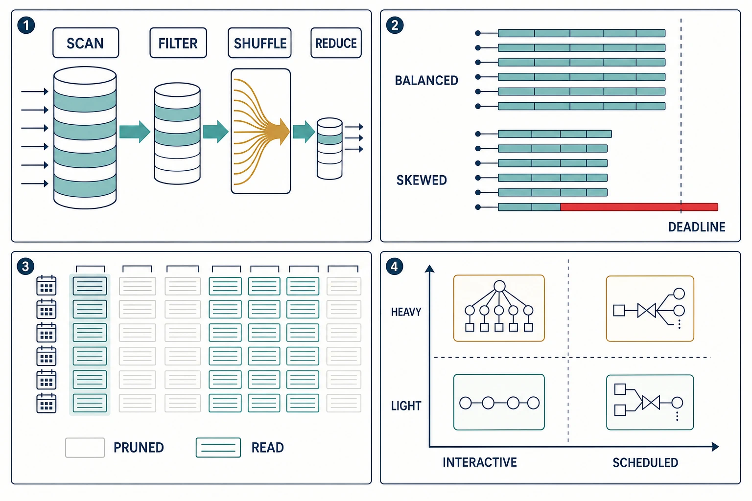
A query plan is a byte-flow graph
A physical plan should make at least four quantities inspectable at every stage:
- input and output rows, including estimate error;
- compressed, decoded, spilled, and transferred bytes;
- task service and wait distributions, including the longest tasks; and
- partition cardinality and size distributions before and after exchanges.
A scan feeds filters and projections. Local partial aggregation may collapse many rows into a small set of group states. A shuffle repartitions records by a join or group key. Reducers combine each key’s state. The arrows are network, serialization, queue, and often disk boundaries—not decorative connectors.
Push reduction before an exchange when the operation is decomposable and preserves semantics. SUM can usually combine partial sums. An average can combine count and sum, not an average of averages without weights. Distinct counts, ordered aggregates, percentiles, user-defined state, and floating-point accumulation need explicit algorithms and error or determinism rules. A partial aggregate that changes null, duplicate, overflow, or ordering semantics is not an optimization.
Join selection depends on the bytes and distribution of both sides after filters, not catalog names. Useful families include:
Broadcast/hash join. Replicate a small build side to workers and scan the large side locally. This avoids repartitioning the large side, but pays replicated network and memory. It is attractive only when the built hash representation fits with reserve on every participating worker.
Partitioned hash join. Repartition compatible keys from both sides and build/probe per partition. It handles two large inputs but pays a shuffle and inherits key skew. Co-partitioned, colocated data can avoid part of that movement if partition functions, versions, counts, and placement genuinely align.
Sort-merge join. Sort or exploit existing order, then merge equal keys. It can fit sequential I/O and range-oriented work but sorting and spill are not free. Existing sort order helps only when filters, collation, null treatment, and key expressions match.
Nested-loop or index-assisted join. Repeatedly probe one side. It can be right for a tiny outer set and selective indexed probes, disastrous when the outer cardinality estimate is wrong, and sensitive to remote round trips.
Planner estimates are hypotheses. Record estimated versus actual rows, bytes, distinct keys, nulls, heavy hitters, and correlation. Sampling that misses a rare but enormous tenant can choose a plan that looks rational and fails exactly on peak day.
Severe skew changes the join decision
SignalWeave must join 2.4 TiB of filtered facts to a 7.5 GiB merchant dimension. The fact join key has 256 shuffle partitions, but one marketplace merchant owns 22% of fact bytes.
average partition = 2.4 TiB / 256
                  = 9.6 GiB

hot partition     = 2.4 TiB × 0.22
                  = 540.672 GiB

hot / average     = 56.32
At a modeled 320 MiB/s of sustained task input, an average partition takes about 30.72 seconds of input service. The hot partition takes about 1,730 seconds, or 28.8 minutes, before other work. More reducers do not split one key if the required output is still keyed to that value.
The first candidate is a broadcast join. Replicating 7.5 GiB to 64 workers transfers 480 GiB but avoids up to 2,457.6 GiB of fact shuffle, a modeled difference of 1,977.6 GiB. A hash-table amplification of 1.65 plus 2 GiB of other working memory requires about 14.375 GiB per worker. It fits the stated 24 GiB available envelope, leaving roughly 9.625 GiB for uncertainty and runtime overhead. That conclusion fails if the 7.5 GiB is compressed-on-disk size rather than built-memory size, if concurrent queries share the worker, or if a worker has less reserve.
If broadcast does not fit, treat heavy hitters separately. A hybrid plan can identify the hot key, replicate only its matching dimension row, split the hot fact rows across 16 deterministic salt buckets, aggregate partials, then merge them. The modeled largest hot shard becomes 33.792 GiB and about 108.13 seconds of input service. Other keys use the normal partitioned join. This plan spends an extra merge and explicit heavy-hitter logic to buy parallelism.
Salting is legal only when the downstream operation can merge partials without changing the answer. A key that requires one globally ordered sequence, a non-decomposable state transition, or a single authoritative side effect cannot be split by wishful hashing. Random salting also needs deterministic replay or a stored salt if reproducibility matters.
The applied decision is therefore conditional:
- verify actual post-filter build bytes and full built-memory footprint;
- if it fits every worker with concurrency reserve, broadcast the dimension and avoid fact shuffle;
- otherwise isolate measured heavy hitters, split only decomposable work, and keep ordinary keys on the cheaper general path;
- if neither is correct, accept the partitioned plan and change the deadline, precompute, or redesign the result.
Speculative execution is not the primary skew repair. It can race a task delayed by a sick worker, transient remote read, or noisy neighbor. Duplicating a deterministic 541 GiB partition creates two expensive copies of the same intrinsic work. Classify a straggler by input size, service rate, wait, spill, locality, retry, and host health before speculating. Cancel the losing copy and account for duplicate I/O.
Memory, spill, and storage locality
Analytical operators use memory for decoded batches, hash tables, sort runs, group state, exchange buffers, code, and the runtime itself. An operator’s resident size is rarely its input file size. Variable-width values, object headers, hash load factor, null maps, dictionaries, and duplicate state can amplify it.
Set an operator memory envelope below the worker limit. When a hash join or aggregation crosses it, a spillable implementation partitions or writes state to storage and later reads it back. Spill converts memory pressure into local or remote I/O, serialization, extra passes, and longer task lifetime. It is a designed slow path, not free elasticity.
Local NVMe can offer high spill bandwidth and low latency but is ephemeral and unevenly occupied. Remote object storage offers durable, elastic capacity but adds request overhead, shared-network demand, and longer tails. A remote shuffle service can decouple intermediate data from worker lifetime, yet adds another service with admission, replication, cleanup, and recovery limits. Choose the boundary by failure semantics and measured service demand, not by the word “local.”
Observe peak operator memory, allocation failures, spill bytes/files/passes, spill read/write throughput, remote throttling, and time blocked on memory. A query that succeeds only by filling the disk is operationally failed if recovery, compaction, or neighboring work needs that disk.
Small files turn metadata into the critical path
Continuous ingestion tends to create many small objects. Four million files averaging 8 MiB represent about 30.52 TiB. If discovery, authorization, footer access, or scheduling spends a modeled 3 ms per file, the serial metadata lower bound is 12,000 seconds. Even 200-way metadata concurrency has a 60-second arithmetic floor before rate limits, retries, and data reads.
Compacting those bytes toward 1 GiB targets yields about 31,250 files. That reduces listings, opens, task scheduling, footer reads, and tiny transfers. It also rewrites data, delays visibility, competes with queries, and creates temporary duplicate bytes. File size must balance scan parallelism, pruning granularity, write cadence, failure recovery, and object-store behavior. “One large file” is not the goal.
Compaction needs ownership and invariants:
- select a closed input range and prevent two compactors from claiming it;
- write new files under a new version or snapshot;
- validate row counts, checksums, partition statistics, schema, and delete application;
- atomically publish metadata that selects the new set;
- retain the old set through reader and rollback horizons; and
- garbage-collect only files unreachable from supported snapshots.
Deletes and updates complicate the lifecycle. Copy-on-write rewrites affected files. Merge-on-read overlays delete or delta files during reads and postpones rewrite cost. Either way, readers need snapshot semantics; otherwise compaction can double count or omit rows during the transition.
Precomputation moves cost across time
A materialized view stores a derived result so readers avoid repeated scans, joins, or aggregates. It exchanges storage, refresh work, lineage, and staleness for query latency. The authority remains named source data unless the view is deliberately promoted to a new authority.
Full refresh is simple but can reread history. Incremental processing applies changes since a known source position or snapshot. It requires stable identities, delete/update semantics, late-data handling, and a recovery path when incremental state is wrong. An incremental aggregate over append-only facts is easier than a join whose dimension corrections must revise years of output.
Choose precomputation when the repeated saved work exceeds refresh and maintenance cost, the result definition is stable enough, and freshness can be expressed. Reject it when query predicates vary so widely that the view rarely prunes work, when correctness requires synchronous source visibility, or when nobody owns reconciliation.
Record view inputs, transform/version, authority, refresh trigger, included source boundary, visible version, freshness objective, rebuild duration, storage, validation query, and consumers. A view that is fast but cannot prove which source state it represents is a cache with an undocumented correctness contract.
Interactive and scheduled work need different queues
One global queue allows a burst of exploratory full scans to delay payroll reporting, or lets scheduled extracts occupy every slot while a human waits for a selective query. Workload management starts by classifying work before admission.
SignalWeave has 64 modeled execution slots: 24 assigned to an interactive pool and 40 to a scheduled pool. Interactive admission permits at most 12 concurrent queries, leaving room for intra-query parallelism; the scheduled pool admits at most 10 concurrent jobs based on predicted peak slots and bytes. These counts are teaching inputs, not a universal ratio.
A useful classification matrix distinguishes:
| class | objective | characteristic work | admission response |
|---|---|---|---|
| interactive-light | subsecond to seconds | metadata, selective lookup, small scan | short bounded queue; reject stale/expensive plan estimates |
| interactive-heavy | minutes with feedback | exploratory join or broad aggregate | explicit heavy lane, lower concurrency, cancel support |
| scheduled-light | finish by dependency time | incremental view or small export | reserve near release; backfill can borrow |
| scheduled-heavy | portfolio deadline and cost | full refresh, training extract, compaction | planned window, byte/slot budget, checkpoint or restart policy |
Queue by deadline and resource shape, not arrival time alone. A job may need scan bandwidth, shuffle bandwidth, memory, and output quota simultaneously. Admission should use conservative predicted work and correct it with observed plan progress. Kill or quarantine a query that exceeds its declared class by a defined factor; do not let optimistic estimates become unlimited authority.
Resource pools provide isolation only if the shared bottlenecks obey them. Separate worker slots do not isolate one object-store account, metadata service, shuffle fabric, catalog, or destination database. Track borrowed capacity, reclaim latency, queue age, deadline risk, and rejected work at each shared boundary.
Cost attribution follows causal work. Attribute scanned bytes, storage requests, transfer, slot or CPU time, spill, materialized-view refresh, compaction, and retries to a workload and owner. Shared base costs can use a documented allocation rule. A dollar total without workload quantities cannot explain a regression; a byte total without price cannot govern economics.
Benchmark the portfolio you actually operate
A single query on uniform synthetic data cannot validate a warehouse. Representative evidence needs data scale and distribution, schema width, compression, partition age, nulls, correlations, heavy hitters, file sizes, deletes, and view state. It also needs a query mix: selective, broad, join-heavy, aggregation-heavy, interactive, scheduled, concurrent, and maintenance work.
Define:
- claim and system boundary;
- engine, runtime, storage format, configuration, hardware, and date;
- data generator or captured fixture, scale, distribution, and allowed sanitization;
- query text and parameters, plan, result checksum, and cache state;
- load arrival, concurrency, warm-up, repetitions, and run order;
- queue, completion, bytes, spill, skew, correctness, and cost measures; and
- known differences from production and the transfer limit.
Cold-cache and warm-cache runs answer different questions. Report them separately. Randomize or balance run order so one alternative does not always receive a warmer system. Validate result equality before celebrating speed. Include compaction, refresh, catalog, and competing queries when they are part of the production state.
TPC-DS provides a controlled decision-support workload with queries, concurrent throughput, and data maintenance, but its result transfers only to the extent that its schema, distribution, scale, query mix, pricing boundary, and benchmark rules resemble the intended claim. Different major versions and scale factors are not casual comparison material. Use a standard workload as a reproducible reference, then retain production-shaped tests for local decisions.
Query review record
Result and objective:
  answer identity/checksum, completion deadline, freshness boundary,
  query/portfolio population, cost envelope

Plan and estimates:
  engine/version, plan hash, estimated versus actual rows/bytes,
  scan/filter/project/join/aggregate/exchange stages

Storage elimination:
  table bytes, selected partitions/columns, row-group/page pruning,
  predicate pushdown, metadata and request counts

Movement and skew:
  local/shuffle/output bytes, partition count/distribution,
  heavy hitters, longest tasks, speculation and duplicate work

Memory and slow paths:
  operator peak, reserve, spill bytes/files/passes, local/remote path,
  failure and restart behavior

Scheduling and economics:
  class/pool, queue and admission, concurrency, borrowed capacity,
  compute/storage/network/request cost and owner

Evidence:
  data/query fixture, correctness oracle, repetitions, cache state,
  raw plans/metrics, uncertainty, production transfer limit

Decision:
  eliminate/move/split/precompute/admit change, rollout guard,
  rollback trigger, next measurement
Reject a review that proposes more workers without stage bytes and partition distributions, claims pruning without actual scanned-byte evidence, compares plans with different answers, or reports completion without queue time and competing work.
Applied work
Choose the skewed join. Using the 2.4 TiB/7.5 GiB model, calculate broadcast transfer and built memory for the real engine. Then obtain actual post-filter sizes and the top-key byte distribution. Decide among broadcast, partitioned, or hybrid heavy-hitter handling. State why salting preserves the answer, how partial results merge, and what happens if the build side grows 2× during peak concurrency.
Reduce scan bytes without changing the answer. Start with one production-shaped query and its result checksum. Record table bytes, files, selected partitions, columns, row groups, and actual bytes read. Make one layout or expression change at a time. Re-run from comparable cache state, confirm result equality, and explain any added write, compaction, metadata, or freshness cost. Success is fewer causal bytes under the same answer and boundary—not a faster run with a different snapshot.
Rehearse contention. Run the morning scheduled mix while injecting a bounded interactive-heavy arrival. Verify pool admission, shared storage/shuffle behavior, deadline reserve, cancellation, and reclaim. A pool that protects CPU while object-store throttling delays every job has not provided portfolio isolation.
Sources and transfer limits
- Apache Parquet file-format documentation describes the portable columnar format and its metadata structures; pruning and pushdown effectiveness depend on the writer, reader, statistics, predicates, and actual files.
- Apache Arrow columnar format specifies adjacency and vectorization-friendly in-memory layouts; it does not guarantee that a query engine uses a vectorized fast path for every type or expression.
- Apache Spark SQL performance tuning documents adaptive plan changes and skew-join handling in Spark; the mechanisms illustrate options, not universal defaults or performance results for other engines.
- TPC current specifications and the TPC-DS workload define a controlled decision-support benchmark. Follow its fair-use and comparability rules; do not transfer leaderboard results to a different workload.
The chapter’s numeric examples are deterministic models in examples/performance-engineering-system-design-handbook/part-05/batch-analytics/. They are not observed benchmarks. The fixture verifies units and internal arithmetic; an operational decision still needs current plan, workload, distribution, hardware, engine/version, concurrency, correctness, and cost evidence.
Decision rule
Optimize bytes read, bytes moved, and straggler work before adding raw compute. Add compute when the remaining plan contains enough independent, balanced work and the shared storage, shuffle, memory, and output boundaries can feed it. Otherwise eliminate work, change placement, split a legal heavy hitter, precompute a stable result, or renegotiate the completion and freshness contract.
Analytical systems turn large retained datasets into bounded completion work. Search systems make a different exchange: they spend indexing and approximation in advance so a small, high-quality answer can arrive inside a user deadline. The next question is not how many bytes can finish by morning, but which candidates deserve the milliseconds that remain.