Performance Engineering and System Design Handbook / Chapter 36
Elasticity, Autoscaling, and Control Loops
Design delayed scaling feedback that protects queue age, useful capacity, recovery reserve, and cost without oscillation.
Preparing audio…
Audio edition
Elasticity, Autoscaling, and Control Loops
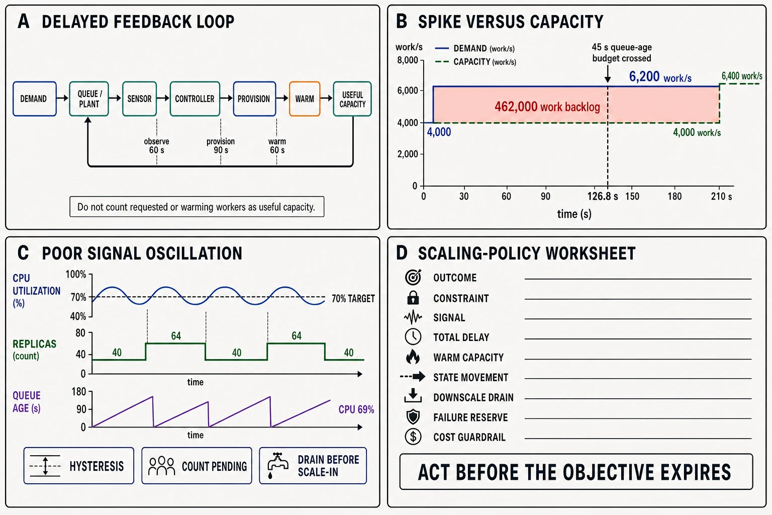
Pulsepipe’s controller log looks calm while its user objective is already doomed:
00:00  demand jumps             4,000 -> 6,200 work/s
00:15  CPU                      69% (target 70%); no action
01:00  queue grows to           132,000 work; add 24 workers
02:30  24 processes exist       readiness=false; warm-up continues
03:30  useful capacity becomes  6,400 work/s
03:30  backlog                  462,000 work
03:30  oldest queued work age     74.5 s
Pulsepipe has 40 warm workers. Each sustains a measured 100 work/s for this mix, giving 4,000 work/s of useful capacity. Intake admits only what the workers can pull, so their CPU remains close to the 70% target even as 2,200 work/s accumulates in a durable queue. CPU is truthful about admitted work and useless as the only signal for waiting work.
The controller observes at 60 seconds, provisioning takes 90 seconds, and warm-up takes 60 seconds. The first useful added capacity arrives 210 seconds after the spike. By then:
deficit = 6,200 - 4,000 = 2,200 work/s
backlog = 2,200 work/s × 210 s = 462,000 work
Pulsepipe’s oldest-work objective is 45 seconds. In a simple FIFO fluid model with uniform work, oldest age grows at the deficit fraction of offered demand: 2,200 / 6,200 seconds per second. The objective is crossed about 126.8 seconds after the spike—well before the new workers become useful. At 210 seconds, the oldest queued work is about 74.5 seconds old. Clearing the 462,000-work backlog at the original service rate would take 115.5 seconds; that drain-time equivalent is not the age of the oldest item.
Autoscaling did not fail to run. It controlled the wrong observation with an actuator slower than the objective.
The governing rule is: scale on the earliest reliable signal of constrained service, while preserving enough headroom to cover detection, provisioning, warm-up, and failure delays.
Read the trace as a feedback system
An autoscaler is a feedback controller around a changing system. Use a small vocabulary:
- plant: the service, queue, runtime, dependencies, and workload whose behavior is being controlled;
- controlled outcome: protected goodput, queue age, lag, latency, or another user-relevant quantity;
- sensor: the measurement and aggregation pipeline;
- setpoint or policy band: the target or acceptable range;
- controller: logic that chooses a capacity recommendation;
- actuator: replica creation, resource resize, admission change, traffic shift, prewarm, or job scheduling;
- disturbance: demand spike, skew, dependency slowdown, regional shift, failure, or noisy neighbor; and
- delay: sampling, export, aggregation, evaluation, API, placement, image pull, initialization, readiness, rebalancing, and load-balancer convergence.
Draw the loop in time order:
demand -> queue/plant -> measured signal -> controller decision
   ^                                            |
   |                                            v
new useful capacity <- warm/register <- provision/placement
The controller acts on a past state. During the delay, demand and backlog continue changing. If it ignores work already requested but not useful, it can request another step each interval and overshoot. If it counts processes before readiness, it can stop too early. If downscale removes warm capacity while the backlog is still draining, the system can oscillate between shortage and excess.
Record one timestamp for every stage:
disturbance detected
metric sampled
metric available
recommendation issued
capacity request accepted
resource placed
process started
workload initialized
representative readiness passed
traffic or partition assigned
first useful completion
steady service demand reached
The useful delay ends at first representative completion, not process creation. A worker that exists but is downloading a model, rebuilding an index, opening connections, replaying a log, or waiting for shard ownership is demand, not capacity.
Capacity, scalability, and elasticity answer different questions
These terms are often collapsed:
- capacity is the safe useful-work envelope of a declared system and workload state;
- scalability describes how behavior and cost change as resources or workload scale across a range; and
- elasticity is the ability to change useful capacity in response to demand within required time, correctness, and economic bounds.
A service can scale nearly linearly from 10 to 100 warm workers and still have poor elasticity if adding one takes 20 minutes. A service can launch processes in seconds and fail to scale because all replicas contend on one database. A large fixed fleet can have ample capacity and no autoscaling.
Define capacity in useful units. “64 pods” is an inventory count. Prefer a scoped statement:
4,000 successful events/s at the declared mix,
oldest queue age <= 45 s,
downstream write p99 <= 120 ms,
correctness checks clean,
one worker class, warmed state, July 2026 environment
Per-instance capacity changes with request mix, payload, cache state, CPU shape, memory pressure, NUMA placement, throttling, network, storage, software version, and dependency latency. Heterogeneous capacity requires weights or direct service-demand estimation. Ten “instances” of two shapes are not twenty equivalent units.
Find the constraint before choosing the actuator. If storage IOPS caps goodput, adding consumers increases contention. If a partition is hot, fleet-wide scale-out may leave its single owner unchanged. If a regional dependency is saturated, traffic shift and local replica growth can amplify it. Scaling is a hypothesis about which added resource releases a constraint.
Choose the earliest reliable constrained-service signal
No universal autoscaling metric exists. Evaluate signals by four properties:
- causal relevance: does the signal represent demand on or saturation of the constrained resource?
- lead time: how long before the controlled objective fails does it move?
- capacity normalization: can the value be translated into required useful capacity across shapes and versions?
- robustness: does missing data, rejection, throttling, cold start, or partial failure make it lie?
Utilization
CPU, memory, network, storage, or accelerator utilization works when the resource is the actual constraint, demand reaches it, and utilization scales predictably with service demand. It fails when admission or a queue hides offered load, when throttling caps measured consumption, when work is I/O-waiting, or when average utilization hides hot workers.
High utilization is not always bad. A bounded batch system may intentionally run near 100% while meeting deadlines. Low utilization is not always safe. One serialized lock, shard, thread, connection pool, or rate limit can constrain goodput while fleet CPU is low.
Concurrency
In-flight work can approximate demand through Little’s Law when boundary and population are stable. Concurrency is useful for request services whose resource exposure grows per active operation. It must separate useful admitted work from abandoned, queued, retry, and blocked work. A concurrency target without deadlines can retain hopeless work.
Queue depth and queue age
Depth measures count; age measures waiting. Age often transfers better when item costs vary or demand changes. Depth can be converted into drain time only with a service-rate model. A low depth containing one expensive or poison item can still violate age; a high depth of cheap background work may be safe.
For Pulsepipe, offered demand is observable at durable enqueue. Queue-age slope reveals a deficit before the 45-second objective fails. The controller uses:
- oldest eligible work age by priority and partition;
- age derivative over a short robust window;
- arrival rate and useful completion rate;
- warm capacity and requested-but-not-ready capacity;
- per-partition heat and downstream saturation; and
- the remaining delay until new capacity can serve.
Consumer lag
Lag in records or offsets is meaningful only with arrival rate and record cost. Ten thousand tiny events differ from ten thousand model-inference jobs. Convert lag into estimated work and drain time, segmented by partition and class. Age of the oldest unprocessed authoritative event is often closer to a freshness objective.
Latency
User latency is decisive evidence but can be a late control signal. Near saturation, latency may rise after queues have already consumed the objective. It is also noisy, mix-dependent, and affected by dependencies the actuator cannot fix. Use latency as an outcome/guardrail and sometimes as a signal when it provides stable lead time—not as the only alarm after violation.
Custom service demand
Estimated CPU ms, storage operations, bytes, accelerator time, or normalized work per logical operation can handle changing request mixes. The estimator needs current calibration and uncertainty. If a new release doubles service demand, an arrival-count target should change before the fleet collapses.
Use multiple metrics asymmetrically. Scale out when any trusted constraint signal demands more capacity; scale in only when all safety signals, backlog, warm-up, failure reserve, and drain state permit it. Missing metrics should normally block destructive scale-in, not protective scale-out.
Controller families are tools, not sophistication ranks
Threshold and step scaling
A threshold triggers a fixed or proportional step when a metric crosses a boundary. It is legible and useful for coarse modes: add a cell, start a standby pool, or enter brownout. One threshold without hysteresis chatters when the signal fluctuates near it. One fixed step underreacts to large disturbances and overshoots small ones.
Define entry threshold, exit threshold, minimum hold, pending capacity accounting, and maximum change per interval. Size the step from deficit and per-unit capacity, rounded with uncertainty:
required units = ceil((forecast demand + reserve - warm useful capacity)
                      / safe capacity per added unit)
“Forecast” can be a short-horizon extrapolation from current rate and queue slope, not necessarily a machine-learning system.
Target tracking
Target tracking attempts to keep a metric such as CPU or work per target near a setpoint. It suits signals roughly proportional to demand per unit and fleets whose units are comparable. It still needs delay handling, minimum/maximum bounds, initialization treatment, and asymmetric scale-in.
A 70% CPU target encodes headroom only if 100% means the relevant safe limit and CPU is the bottleneck. It does not reserve database IOPS, cover a cold cache, or protect a regional failure. The target should come from load tests and recovery requirements, not a round number.
Predictive and scheduled scaling
Scheduled capacity is appropriate for known launches, market opens, backups, daily peaks, or batch windows. Predictive control uses historical patterns and leading indicators. Both act before a slow actuator, which is valuable when T_provision + T_warm exceeds the objective.
Prediction is uncertain. Keep reactive correction, admission, and bounds. A forecast trained on ordinary weekdays will miss a product launch or incident-driven traffic shift. Track forecast error by horizon and cost false positives separately from shortage.
Event-driven scaling
Events such as queue arrival, partition creation, job submission, or a regional evacuation can trigger capacity requests. An event is early but may not represent cost. Deduplicate triggers, aggregate bursts, cap actions, and validate whether downstream capacity exists. The arrival event can also prewarm before backlog age rises.
Combine modes deliberately. Pulsepipe maintains a scheduled base for predictable traffic, an event-driven prewarm on launch markers, queue-age reactive scale-out, and slow evidence-based scale-in. Four controllers without ownership, precedence, and shared pending-capacity state would fight.
Delay determines the safe policy band
Let:
λ= offered demand in work/s;μ= current useful capacity in work/s;d = max(0, λ - μ)= deficit in work/s;T= time until added capacity becomes useful in seconds; andB_0= current backlog in work.
A simple lower-bound backlog projection is:
[ B_T = B_0 + dT ]
It assumes fixed demand and capacity, no retries, and equivalent work. It is not a queueing forecast, but it can disqualify a controller.
For an initially empty FIFO queue with uniform work, the corresponding oldest-work age is:
[ A_T = T\left(1 - \frac{\mu}{\lambda}\right) = T\frac{d}{\lambda} ]
Pulsepipe has d = 2,200 work/s and T = 210 s, so B_T = 462,000 work and:
[ A_T = 210 s \times \frac{2,200}{6,200} \approx 74.5 s ]
Its 45-second oldest-work objective crosses after:
[ T_{cross} = 45 s \times \frac{6,200}{2,200} \approx 126.8 s ]
This age relation depends on FIFO service, uniform work, and an initially empty queue. With priorities, partitions, variable work, retries, or an existing backlog, measure age directly by class and use the backlog projection only as a separate capacity bound.
The policy cannot meet the objective by waiting for the first 60-second observation and then cold-provisioning for 150 seconds. Viable changes include:
- keep enough warm headroom that the deficit stays inside the queue-age budget;
- prewarm from a schedule or leading event;
- sample and decide earlier;
- reduce provisioning/warm-up time;
- increase safe per-unit capacity;
- shed/defer lower-priority work at admission;
- route to already warm reserved capacity; or
- change the user objective with product approval.
Adding 24 workers raises modeled capacity to 6,400 work/s, only 200 work/s above sustained 6,200 demand. Draining 462,000 work at a net 200 work/s takes 2,310 seconds, or 38.5 minutes, if demand stays flat. “Caught up to current demand” is not “recovered.” A larger temporary step may drain sooner but must fit dependencies and cost.
Model the full response:
T_effect = T_sample + T_export + T_evaluate + T_api
         + T_place + T_start + T_warm + T_assign

recovery time ~= T_effect + backlog / (new useful capacity - live demand)
When the denominator is zero or negative, scale-out stabilizes the backlog but never drains it.
Oscillation is usually a causal clue
Oscillation means capacity, signal, or traffic repeatedly crosses policy boundaries. Common causes include:
- measurement arrives after the state it represents;
- controller ignores requested/pending capacity and repeats the action;
- newly started workers report misleading startup utilization;
- load balancing shifts too quickly to cold workers;
- scale-out lowers average utilization below the scale-in threshold before backlog drains;
- scale-in removes caches/connections and raises service demand;
- multiple autoscalers act on the same plant;
- traffic steering and regional scaling chase each other; or
- a dependency limit makes added replicas increase latency rather than capacity.
Hysteresis uses different expand and contract boundaries. A policy might begin expansion when projected queue age at T_effect exceeds 30 seconds, but permit contraction only after age remains below 5 seconds, useful capacity is stable, and reserve passes for 15 minutes. The values come from delay, noise, and objective evidence.
A stabilization window considers recent recommendations so one low sample does not reverse a prior high need. A cooldown controls how quickly another action occurs. Neither should be folklore. A cooldown shorter than warm-up can issue duplicate actions; one longer than the time-to-objective can prevent necessary correction. Track pending capacity explicitly rather than relying only on a timer.
Use rate limits on actions: maximum units or percentage per interval, minimum meaningful step, and maximum fleet. Rate limits contain controller defects but can also make a correct controller too slow. Verify both protection and reachability under the largest credible disturbance.
Jitter can decorrelate thousands of controllers polling or replacing at once. It must not randomize safety bounds or make an operation miss its deadline. Seeded jitter improves replayability.
Scale out and scale up change different constraints
Scale out adds parallel workers. It improves capacity when work partitions, dependencies scale, and coordination does not dominate. It can add connections, replicas, cache misses, leader elections, scheduler pressure, and fan-out.
Scale up gives a worker more CPU, memory, bandwidth, accelerator capacity, or storage performance. It preserves locality and avoids partition movement, but may require restart, be coarse, hit shape ceilings, or reduce failure-domain count.
Compare by bottleneck and time:
| pressure | scale out may help when | scale up may help when | hidden cost |
|---|---|---|---|
| stateless CPU | requests are independent and downstream has room | per-process parallelism and shape change are efficient | cold code/cache, connections |
| memory working set | data can partition or replicate economically | locality is valuable and larger memory avoids misses | redistribution or restart |
| hot partition | key can split or ownership can move | owner benefits from a larger shape | migration, fencing, skew |
| storage throughput | requests distribute across independent paths | volume/device supports online resize | compaction, rebuild, shared limit |
| accelerator inference | batches route across devices | model needs more memory or one larger device | model load, scheduling, cost |
A controller may choose both: vertically resize a hot stateful shard and horizontally add stateless readers. Record which action is reversible, its delay, and its authority implications.
Stateful scaling is a migration controller
Adding a stateless process can be fast. Adding useful stateful capacity may require partition creation, snapshot transfer, log catch-up, index build, checksums, authority transfer, cache warm-up, and rebalancing. These consume the constrained storage and network resources.
Separate phases:
- allocate resource;
- seed state under a bandwidth/IO budget;
- catch up while live writes continue;
- validate state and schema;
- assign a bounded read fraction;
- transfer authority with a fenced epoch if needed;
- rebalance incrementally; and
- verify goodput, skew, and recovery reserve.
Count a shard as capacity only when it can perform representative work. During movement it may reduce net capacity. Autoscaling based on lag can create a positive loop: lag requests consumers; consumers trigger rebalances; rebalances pause consumption; lag rises; more consumers are requested.
Use stable partition assignment, minimum residence time, movement budgets, and separation between compute and ownership decisions. Sometimes adding consumers without adding partitions has no effect. Sometimes splitting the hot partition is the only relevant action.
Backfill and replica repair need their own admission. Foreground scaling should not unlock unlimited state movement. Coordinate with Chapter 34’s recovery workload and Chapter 35’s regional bandwidth/reserve model.
Downscale is a drain protocol
Scale-in destroys optional capacity and can interrupt accepted work. A safe decision proves:
- backlog and oldest age are below contraction thresholds;
- arrival/service-demand uncertainty fits remaining warm capacity;
- failure and regional reserve remains intact;
- no pending scale-out or traffic shift is hidden;
- dependencies will not become the new constraint;
- selected workers can stop admission;
- long-lived sessions, streams, leases, and shard ownership can move;
- in-flight work becomes terminal, handed off, or queryable; and
- cache loss and reconnection cost are included.
The sequence is:
select removal target -> stop new assignment -> propagate routing change
-> transfer durable ownership -> drain to bound -> force stop if required
-> observe remaining fleet through a stability window
Do not choose victims only by lowest CPU. They may hold rare warm state, tenant affinity, a partition, a local cache, or the only healthy connection path. Rank by removal cost and failure-domain balance.
For queue workers, stop leasing new work, finish or safely release current leases, preserve effect identity, and avoid acknowledging incomplete effects. For request servers, close admission, drain connections within deadlines, and ensure retries do not amplify remaining replicas. For stateful owners, advance authority epoch before accepting work elsewhere.
Keep a minimum warm floor derived from boot delay and demand uncertainty. If zero-to-one takes five minutes and the user objective is 45 seconds, scale-to-zero is only valid for work that can wait or when an earlier event prewarms reliably.
Cold starts are both latency and load
Initialization may include resource placement, image pull, runtime/JIT, model or index load, configuration, key/certificate retrieval, DNS, connection establishment, cache fill, shard sync, and readiness. Each step has a distribution and dependencies.
Cold starts can manufacture overload:
- many workers fetch the same image or model;
- connection storms hit a database;
- empty caches transfer reads to authority;
- JIT/initialization consumes CPU counted as user demand;
- readiness flips before representative state is warm; and
- retrying initialization synchronizes the fleet.
Prewarming moves this work earlier. Options include warm pools, minimum replicas, scheduled start, snapshot/restore, lazy bounded loading, image locality, connection ramp, cache seed, and probation traffic. Prewarming costs money and can carry stale state; validate versions and credentials.
Measure start-to-process, process-to-ready, ready-to-first-useful-completion, warm-up service demand, failure rate by stage, and effect on dependencies. Use quantiles by shape, image, zone, and version. A median warm-up is not a safe control delay.
Headroom and failover reserve are policy, not idle waste
Headroom absorbs forecast error, sampling delay, skew, failures, recovery work, and controller mistakes. Separate:
- routine elasticity headroom: covers demand until the actuator responds;
- failure reserve: covers declared node/zone/region loss;
- recovery reserve: funds replay, refill, repair, and state movement; and
- uncertainty margin: covers model error and variance.
Do not count one unit twice unless modes are mutually exclusive and that assumption is defended. Capacity used for ordinary peak scale-out is unavailable for regional evacuation at the same moment.
Pulsepipe protects 5,000 work/s and reserves 20% for a declared failure envelope:
required warm capacity = 5,000 × 1.20 = 6,000 work/s
available warm capacity                    6,400 work/s
modeled margin                               400 work/s
That 400 work/s is not automatically safe for background jobs. It may cover mix variance, probes, control traffic, or a second disturbance. Test the degraded mix and every dependency.
A regional traffic evacuation can instantly increase offered load in the destination while its local autoscaler also sees a spike. Do not assume remote traffic shift, local scale-out, cache warm-up, and database capacity are independent. Pre-reserve or prewarm receiving capacity, cap the route ramp, and exchange explicit capacity state between controllers.
Cost-aware scaling needs a service objective
Autoscaling optimizes an economic objective under safety constraints. Cost per provisioned unit is incomplete. Track cost per successful, useful, objective-compliant operation, including idle reserve, startup, state movement, egress, license, energy, and operator complexity.
A cost-aware policy can:
- use scheduled base capacity for predictable demand;
- buy flexible capacity for uncertain bursts;
- place interruptible work on preemptible resources;
- shift deferrable jobs into cheaper windows;
- choose vertical versus horizontal shapes by measured cost frontier;
- shed low-value work when marginal capacity exceeds value; and
- reduce capacity slowly after stability and drain.
Spot or preemptible resources are uncertain capacity. They suit replayable, checkpointed, redundant, or deferrable work with interruption-aware scheduling. They should not constitute the only failure reserve. Model correlated revocation, replacement delay, checkpoint/write amplification, and loss of multiple instances.
Predictive overprovisioning has a cost; reactive shortage has user and recovery cost. Record both. The controller can minimize expected cost only after minimum goodput, latency/age, correctness, and reserve constraints are hard gates.
Avoid cross-region price chasing for authority-sensitive state without including latency, egress, residency, migration, and disaster posture. Cheap compute can produce expensive coordination.
Observe the controller as production software
Controller telemetry must make cause reconstructable:
- raw and aggregated input metrics with sample/event time;
- missing/stale metric decisions;
- desired, requested, starting, warming, ready, draining, and failed capacity;
- recommendation by each policy and final arbitration;
- action timestamps and provider/scheduler responses;
- per-unit capacity calibration and version;
- queue depth, oldest age, arrival, completion, and protected goodput;
- dependency saturation and rejection;
- forecast plus error bands;
- reserve consumption by mode;
- scale event reason, owner, and correlation ID; and
- manual overrides with expiry.
Graph demand, useful capacity, pending capacity, backlog/age, objective, and controller actions on one aligned time axis. Average CPU alone cannot explain a control failure.
Alert on controller pathologies: recommendation cannot actuate, warm-up exceeds bound, pending capacity grows without readiness, scale events alternate repeatedly, reserve falls below policy, backlog grows after scale-out, scale-in increases service demand, or a metric disappears while contraction continues.
Version policies and treat changes like code. Replay historical and synthetic traces through the decision logic, simulate missing/delayed metrics, shadow recommendations, canary one cell, limit velocity, and preserve rollback. A syntactically valid policy can destabilize a fleet.
Scaling-policy worksheet
Controlled outcome:
  population, mode, goodput/latency/queue-age objective

Plant and constraint:
  unit of useful work, workload mix, bottleneck, per-unit capacity distribution

Signals:
  raw metric, boundary, aggregation, sampling/export delay, lead time,
  missing/stale behavior, normalization, known false signals

Actuators:
  scale out/up, prewarm, route, admit/shed; min/max/step/rate;
  provisioning, warm-up, assignment, and first-useful-work distributions

Controller:
  reactive/predictive/scheduled/event-driven; setpoint/bands;
  hysteresis, pending-capacity accounting, stabilization, arbitration

Stateful cost:
  snapshot, catch-up, rebalance, fencing, cache/connection warm-up

Scale-in:
  evidence window, victim selection, drain/ownership protocol, force bound

Reserves:
  routine delay, failure, recovery, uncertainty; no double counting

Economics:
  cost per objective-compliant operation, capacity class, interruption risk

Validation:
  trace replay, simulation, load/fault test, shadow/canary, abort, rollback
Reject a policy whose controlled outcome is merely replica count, whose signal moves after the objective, whose actuator delay is unknown, or whose downscale cannot prove ownership.
Control-loop drills
Classify the claim. “We can handle 8,000 work/s,” “throughput doubles from 10 to 20 workers,” and “we add safe capacity inside 90 seconds” are capacity, scalability, and elasticity claims respectively. Add workload, state, objective, range, and evidence to each.
Reproduce the trace. Calculate 4,000 work/s initial capacity, 2,200 work/s deficit, 210-second effect delay, 462,000-work backlog, 74.5-second oldest age, and 126.8-second objective crossing under the stated FIFO fluid model. Then vary the first observation from 60 to 15 seconds and warm-up from 60 to 20 seconds. Decide whether the 45-second objective becomes feasible without prewarmed headroom.
Rank signals. For CPU-bound stateless API, IOPS-bound database, queue-backed worker, and hot single partition, rank utilization, concurrency, depth, age, lag, latency, and service demand. Name the actuator each signal can actually influence.
Repair CPU-only scaling. Intake throttling keeps CPU at 69% while queue age rises. Add a queue-age projection, arrival/completion rates, pending-capacity state, downstream guardrail, and admission response. Explain why simply lowering CPU target may still fail.
Stabilize oscillation. A fleet alternates 40 and 64 workers every eight minutes. Align metrics and actions, inspect startup samples and scale-in timing, set evidence-based hysteresis, and prove that the revised policy still responds before the objective.
Scale state safely. Add two storage shards under a write-heavy workload. Budget copy/apply traffic, avoid rebalance thrash, fence authority, and state when each shard begins counting as useful capacity.
Downscale under streams. Remove 20% of workers holding long-lived sessions and message leases. Specify admission stop, connection drain, lease/effect handling, maximum grace, and queryable interrupted outcomes.
Red-team cheap capacity. Half the fleet uses preemptible instances and a regional event simultaneously increases demand and revocations. Prove protected warm reserve, route-ramp bounds, interruption handling, and a cost threshold that never overrides the objective.
Durable rules for elasticity
- State capacity, scalability, and elasticity separately, with workload, state, range, and objective.
- Control a user-relevant outcome and identify the constrained resource before selecting an actuator.
- Choose the earliest reliable signal; CPU is only valid when CPU demand is exposed and constraining.
- Sum measurement, provisioning, warm-up, assignment, and first-useful-work delays.
- Project backlog and time-to-objective during actuator delay; reject policies that cannot arrive in time.
- Count requested, starting, warming, and draining capacity separately from useful warm capacity.
- Use hysteresis, stabilization, rate limits, and shared pending-capacity state to prevent reversal and duplicate action.
- Treat stateful scale-out as a migration that consumes resources and may temporarily reduce capacity.
- Treat downscale as an ownership-and-drain protocol, not process deletion.
- Preserve distinct routine, failure, recovery, and uncertainty reserves without double counting.
- Make predictive, scheduled, event-driven, and reactive controllers explicit about precedence and uncertainty.
- Optimize cost per objective-compliant operation only inside correctness, goodput, latency/age, and failure gates.
Capacity control determines who gets resources next. In a shared system, aggregate stability can still conceal one tenant consuming queues, cache, storage, and tail budget. The next design boundary is therefore ownership and fairness: measuring demand per tenant and containing noisy neighbors without wasting the pool.
Evidence and transfer limits
- Official Kubernetes Horizontal Pod Autoscaling documentation describes an intermittent control loop, configurable metrics, not-yet-ready handling, scaling behavior, and stabilization. Defaults and mechanics are version-sensitive implementation examples, not universal controller constants.
- Official AWS target-tracking documentation describes targets and service-specific cooldown behavior. A provider cooldown does not replace measurement of Pulsepipe’s plant, warm-up, or queue-age budget.
- Google’s primary Autopilot paper reports one production approach to horizontal and vertical resource configuration using historical data and heuristics. Its fleet results do not transfer without workload, policy, and environment evidence.
- The executable fixture in
examples/performance-engineering-system-design-handbook/part-04/autoscaling-control/reproduces the fixed-delay step model, FIFO oldest-age estimate, drain time, and reserve arithmetic. It intentionally omits variable arrivals, service-time distributions, retries, priorities, failures, and nonlinear dependencies; use trace replay, simulation, load tests, and staged production evidence before setting a real policy.