Performance Engineering and System Design Handbook / Chapter 23
Load Balancing and Work Placement
Choose placement boundaries, cost signals, locality policies, and control loops that bound skew without creating churn or failure amplification.
Preparing audio…
Audio edition
Load Balancing and Work Placement
Every Mercury worker receives 1,500 requests per second. The request-count dashboard is perfectly flat. Yet two workers exceed their modeled CPU budget while six have headroom, and fleet-average CPU says the service has capacity to spare.
The requests are not equal work. One may decode a 2 KiB object and use 0.2 ms of CPU; another may decompress 200 KiB, fetch remote state, and use 18 ms. The cost range in Mercury’s workload is 90×, and costly request classes are correlated with destinations. Round robin distributes arrival count, not service demand. Sticky placement may preserve reusable state while deepening the skew. A least-loaded policy may help, but only if its observation is timely and measures the resource that constrains the work.
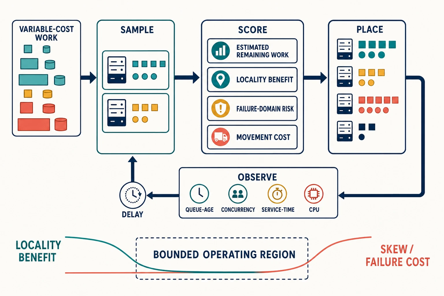
Before choosing among them, name the unit being placed, the resource demand being balanced, and the cost of leaving a preferred destination. Placement is a constrained estimate of future cost, not a count-spreading trick. A good policy uses enough information to bound queueing, skew, locality loss, failure exposure, and movement—without spending more on measurement and control than the imbalance costs.
Define the placement decision before choosing an algorithm
A placement record needs five boundaries:
- Unit: packet, connection, request, task, partition, object, batch, actor, or tenant.
- Destination: thread, process, host, shard replica, rack, zone, region, or accelerator.
- Decision lifetime: one operation, one connection, one session, one lease, or a durable ownership epoch.
- Demand vector: CPU time, bytes read, memory residency, accelerator time, I/O operations, locks, downstream calls, or a learned/synthetic cost.
- Constraints: health, correctness, data authority, locality, tenant isolation, topology, and failure-domain rules.
“Balance” without those fields has no denominator. A packet distributor and a partition scheduler may both use hashing, yet their movement costs differ by orders of magnitude. Reassigning an unstarted stateless request costs a routing decision. Moving a 2 TiB stateful partition consumes network and storage bandwidth, warms caches, changes ownership, and creates a recovery window.
Represent a candidate destination (i) with a scoped score:
[ S_i = \widehat{W_i} + \widehat{D_{r,i}} - L_{r,i} + F_i + M_{r,i} ]
where:
- (\widehat{W_i}) is estimated remaining work already assigned to destination (i), in a declared resource unit;
- (\widehat{D_{r,i}}) is estimated demand of request or task (r) at (i);
- (L_{r,i}) is a measured locality credit, such as avoided remote bytes or warm-state service time;
- (F_i) is a failure-domain or policy penalty; and
- (M_{r,i}) is the immediate and deferred movement cost.
The terms do not need to collapse into one magical scalar. Hard constraints should remain hard: do not place a write on a read-only replica merely because its queue is short. For viable candidates, a lexicographic rule can first preserve authority and failure-domain constraints, then minimize deadline risk, then compare demand and locality. The equation is a review aid: it exposes which costs a simpler policy ignores.
Every estimate has a scope and age. A queue length observed 80 ms ago may be useless for 2 ms jobs. CPU averaged over a minute cannot steer millisecond requests. A request-cost predictor trained on successful warm requests may underprice cold, failed, or adversarial cases. The placement design must therefore include the measurement window, propagation delay, missing-data behavior, and fallback policy.
Static placement and dynamic placement solve different problems
Static placement derives a destination from stable inputs: a configuration map, partition ID, tenant, key hash, topology rule, or fixed weight. It is cheap, explainable, and resistant to fast feedback noise. It can preserve affinity and make state ownership legible. It reacts slowly—or not at all—to a straggler, hot key, changing request mix, or temporary capacity loss.
Dynamic placement incorporates current observations such as in-flight work, queue age, service time, or health. It can avoid transient hot spots and heterogeneous antagonist load. It also creates a feedback controller. Observation, dissemination, selection, execution, and measurement all take time. Too many independent schedulers can chase the same apparently idle destination, overload it, then flee together.
Most production designs combine the two:
- static constraints define eligible destinations and preferred locality;
- bounded sampling avoids global state collection;
- dynamic signals choose among a small eligible set;
- weights represent slower capacity differences;
- hysteresis and minimum residence time prevent churn; and
- a conservative fallback remains usable when telemetry or the controller is unavailable.
The static layer answers “where may this work run?” The dynamic layer answers “which eligible destination is least likely to violate the objective now?”
Policy comparison under variable task size
No policy dominates without a workload. The following table treats each row as a mechanism, not a product setting.
| policy | state needed | strength | characteristic failure | best evidence |
|---|---|---|---|---|
| round robin | ordered healthy set | low overhead; fair arrival count over time | ignores variable cost, long-lived connections, and capacity differences | per-worker arrivals and demand distributions |
| weighted round robin | healthy set plus slow-changing weights | represents known heterogeneous capacity | stale weights and request-mix changes recreate skew | completed demand per capacity unit |
| uniform random | healthy set | decentralized and correlation-resistant | random variance; no demand or locality signal | assignment variance and tail queues |
| power of two choices | two sampled candidates plus comparable load | large improvement over one random choice in idealized allocation models | sampled signal can be stale or incomparable; affinity can be lost | candidate-sample age and post-choice queue/work |
| least loaded | broad current load view | responds directly to observed imbalance | herd behavior, telemetry cost, feedback delay, dishonest load signal | decision-to-effect delay and oscillation |
| least outstanding / least request | in-flight counts | inexpensive proxy when service demands are similar | long and cheap requests count equally | in-flight count stratified by request class and service time |
| estimated remaining work | queue plus per-class remaining demand | matches variable service demand more directly | prediction bias, censoring, multi-resource mismatch | prediction error and objective by class |
| affinity or consistent placement | stable key and membership | preserves cache/data locality; limits remapping | hot keys, uneven key demand, failed sticky destination | key-level demand, miss/remote cost, remap volume |
The classic power-of-two result concerns stylized balls-and-bins allocation. Its durable lesson is that a small amount of choice can be disproportionately valuable; it does not prove that two stale CPU samples solve a multi-resource service. Candidate selection, load definition, task-size distribution, and eligibility still determine transfer.
Google’s published data-center load-balancing discussion describes production cases where the most expensive requests consume far more CPU than the cheapest. Its modern Prequal work similarly emphasizes estimated latency and requests in flight rather than “CPU balance” as an end in itself. These are useful production observations, not universal endorsements of one signal.
Connection balance is not request balance
A connection-level balancer chooses an endpoint when a transport connection is established. The endpoint may then receive thousands of requests, multiplexed streams, or a long-lived session. This preserves connection state and avoids per-request routing overhead, but later traffic cannot be redistributed without opening or migrating connections.
The teaching fixture has 100 connections. Ten hot connections carry 70% of traffic. Each hot connection therefore carries seven times the mean connection’s traffic share. Equal connection counts across workers can be badly unequal request rates, bytes, CPU, and queueing. HTTP multiplexing can make connection count an even weaker proxy because one connection can carry many concurrent streams.
Request-level balancing sees each request and can react to cost class, deadline, queue state, and health. It pays per-request policy cost, may cross locality boundaries, and must preserve request semantics. Streaming, connection-bound authentication context, transaction state, or ordered session behavior can restrict routing.
A common composition is connection-level distribution to a stateless frontend tier, then request- or task-level placement behind it. Observe both boundaries. If the frontend reports even connections while backend queues diverge, the first balance metric has not falsified the second imbalance.
Choose a signal that predicts the scarce resource
Queue length is meaningful only with job sizes. Ten 0.2 ms requests are less work than one 18 ms request. Queue age directly reveals how long admitted work has waited, but it reacts after delay appears and can be distorted by priority or cancellation. In-flight concurrency approximates pressure when jobs have similar resource shape; it underprices expensive or blocked work. Service time can estimate demand, but observed response time includes queueing and may create a self-reinforcing penalty against already-busy workers.
CPU is tempting because saturation is visible. It has four limits:
- host CPU mixes this service with neighbors and kernel work;
- a service can be constrained on memory bandwidth, locks, I/O, or downstream concurrency before CPU saturates;
- utilization says how busy a resource was, not how much assigned work remains; and
- smoothing and collection delay can outlive the jobs being placed.
A synthetic cost can be better when request features predict demand: records scanned, pixels decoded, query operators, input tokens, projected output tokens, bytes decompressed, or fan-out width. Price the feature in the unit of the current constraint. Re-estimate by class and state—warm/cold, cache hit/miss, successful/failed—because a single average teaches the scheduler to ignore tails and phase changes.
For multi-resource work, use a vector or dominant-resource rule. A GPU-memory-heavy request and a compute-heavy request can coexist even when either scalar “cost” appears high. Conversely, placing two jobs with different scalar prices may still collide on the same memory bandwidth or lock. The placement review should name the resource that each cost dimension protects.
Applied diagnosis: balanced counts, skewed CPU
Mercury receives a modeled 12,000 requests/s:
| class | rate | modeled CPU/request | modeled CPU demand |
|---|---|---|---|
| catalog read | 9,000/s | 0.2 ms | 1,800 ms/s |
| personalized read | 2,400/s | 2 ms | 4,800 ms/s |
| portfolio reprice | 600/s | 18 ms | 10,800 ms/s |
| total | 12,000/s | — | 17,400 ms/s |
The request-cost range is 90×. Eight workers average 2,175 ms of CPU demand per second, below a modeled per-worker budget of 3,000 ms/s. A count-balanced assignment nevertheless produces this demand vector:
worker             A     B     C     D     E     F     G     H
requests/s      1500  1500  1500  1500  1500  1500  1500  1500
CPU ms/s        5100  3900  1600  1500  1450  1350  1250  1250
budget          3000  3000  3000  3000  3000  3000  3000  3000
Two workers exceed the budget while fleet mean utilization is 72.5% of that budget. The cause is not insufficient aggregate CPU in this model; it is correlation between costly request classes and destinations.
Repair the policy in stages:
- Classify requests using features known before expensive work begins.
- Seed each class with measured CPU-service distributions, not response time.
- Track queued remaining cost per worker; decrement from observed progress or completion.
- Sample two eligible workers and choose the smaller predicted remaining demand, preserving hard authority/topology rules.
- Correct estimates online by class and state, while bounding any single prediction.
- Compare predicted versus observed demand and keep a simple weighted-random fallback.
The fixture’s modeled work-aware vector peaks at 2,250 ms/s and leaves every worker under budget. This arithmetic proves only internal consistency. A rollout must show per-class queue age and p99, prediction error, CPU service, other resource pressure, rejection, and useful completions. If memory bandwidth becomes the next constraint, the CPU-cost policy needs another dimension.
Locality is a credit, not a veto
Affinity can preserve a parsed object, compiled plan, model weights, connection, CPU cache, filesystem page, or application cache. It can reduce remote bytes and improve service time. It can also concentrate a tenant, hot key, or failure domain; keep sessions attached to a slow worker; and turn a machine loss into a large cold-start event.
Measure locality as avoided work:
- cache-hit or remote-read probability by key/class;
- bytes and service time avoided when local;
- warm-up time and memory retained;
- skew introduced by the affinity group;
- remapping and recovery work after loss; and
- correctness implications of state authority.
Sticky sessions deserve special suspicion. If stickiness exists only because application state lives in one process, it may be coupling disguised as optimization. If a stateful protocol or expensive warm model genuinely needs affinity, specify how a failed or draining worker releases the lease and how the replacement rebuilds state under a bounded budget.
Locality-versus-balance frontier
The fixture provides three modeled operating points:
| policy | max worker CPU | remote reads | state movement | interpretation |
|---|---|---|---|---|
| strict affinity | 3,400 ms/s | 0 MB/s | 0 GiB/min | locality wins; worker budget is violated |
| bounded affinity | 2,450 ms/s | 120 MB/s | 2 GiB/min | preserves affinity until a work bound is crossed |
| balance first | 2,250 ms/s | 350 MB/s | 9 GiB/min | lowest CPU skew; much more remote and migration work |
The middle point is attractive only if 120 MB/s and 2 GiB/min fit network, cache, recovery, and cost budgets. The table is a frontier, not a ranking. If remote reads add 40 ms to a strict p99 objective, more local CPU headroom may be cheaper. If an affinity group can lose an entire rack, modest steady-state remote work may buy safer failure behavior.
Slow workers, stragglers, and outlier ejection
A slow worker may be saturated, throttled, paused, cold, contending, paging, waiting on a dependency, or processing an expensive but legitimate job. A straggler is an observation relative to a comparable cohort and request class—not a moral judgment about a host.
Outlier ejection can protect new work from a destination whose recent error or latency evidence exceeds a policy threshold. It does not repair that destination. Ejection also shrinks available capacity and shifts work to peers. If every worker slows because a dependency is failing, ejecting them in sequence can convert a shared slowdown into total unavailability.
Design ejection with:
- a minimum sample count and comparable request classes;
- success, error, deadline, and service-time signals separated from queue time;
- bounded ejection percentage per locality/failure domain;
- exponential or staged re-entry rather than synchronized return;
- probe traffic that does not falsely certify only a cheap path;
- capacity checks before transferring load; and
- an admission response when the remaining fleet cannot carry demand.
Hedging and duplicate execution can reduce some straggler tails, but they create extra demand precisely when the system may be constrained. Chapter 25 treats their deadline and idempotency contract. Placement should expose the evidence required to decide, not silently duplicate work.
Consistent placement limits churn; it does not guarantee balance
Hash-based placement maps a stable key to an eligible destination without consulting global instantaneous load. Simple modulo assignment, (hash(key) \bmod N), remaps most keys when (N) changes. The fixture contrasts a modeled 10-to-11 worker change: modulo assignment has a 10/11 expected remap fraction under uniform independent hashes, whereas a minimal-disruption scheme aims near 1/11. Actual movement depends on the algorithm, key distribution, replicas, weights, and membership transition.
Consistent hashing and rendezvous-style schemes make membership churn tractable, especially for connection affinity, caches, and partitions. They do not make key demand uniform. A single key can dominate load. Virtual nodes and weights can smooth aggregate assignment, but heavy keys still need replication, splitting, request coalescing, or bounded overflow.
Bounded-load consistent hashing adds an explicit capacity ceiling and redirects assignments that would exceed it. The cited research gives theoretical guarantees under its model. A production adaptation must define “load” (keys, bytes, request demand, or state), capacity weights, overflow search, concurrent membership views, and movement semantics. The bound can trade locality for balance; record both.
Maglev is a useful connection-aware example: its published design combines a consistent lookup table with connection tracking to limit disruption. That does not make its data structure a universal scheduler for stateful partitions or variable-cost application requests.
Topology is part of correctness and recovery
Spreading replicas across racks or zones reduces correlated loss only if the placement policy knows the topology and the failure model is credible. Balancing traffic equally across three zones at high utilization can still fail the evacuation test.
With three equal zones at 60% steady utilization, losing one transfers the same work onto two zones:
[ U_{after} = 0.60 \times \frac{3}{2} = 0.90 ]
The modeled post-loss utilization is 90%, before cold caches, reconnections, re-replication, or degraded hardware. At 70% steady utilization it would be 105%: no placement algorithm can fit that work without admission, degradation, or additional capacity.
Topology rules should cover:
- steady traffic and state placement;
- failover headroom by failure domain;
- cross-zone/region latency and transfer cost;
- quorum or authority constraints;
- evacuation order and partial connectivity;
- re-entry rate after recovery; and
- telemetry grouped by both destination and source locality.
Region placement additionally confronts physics, data residency, and consistency. Do not conceal a synchronous cross-region critical path behind a low regional CPU average.
Heterogeneous capacity requires measured weights
A worker with twice as many cores is not necessarily a 2× worker. Memory bandwidth, NUMA layout, accelerator type, clock policy, thermal state, storage, network, and workload vector alter effective capacity. Derive weights from sustainable useful demand under the target mix and objective, not instance labels.
Weights should change more slowly than per-request load signals. A weight captures baseline capacity; queued remaining work captures current commitment. Combining both avoids sending equal demand to unequal machines or treating a temporarily idle small worker as equivalent to a large one.
Normalize a candidate’s remaining work by its measured capacity:
[ P_i = \frac{\widehat{W_i} + \widehat{D_{r,i}}}{C_i} ]
Here (C_i) is sustainable demand per second for the relevant workload and state. The ratio is predicted pressure, not generic utilization. Revalidate weights after runtime, hardware, power, compiler, request-mix, or locality changes. During mixed-fleet rollout, cap exposure so an optimistic new weight cannot overload one hardware class.
Centralized and decentralized schedulers pay different coordination costs
A centralized scheduler can enforce global constraints, reservations, topology, and placement history. It can plan expensive state movement and explain why a destination was chosen. Its state may be delayed; the service can become an availability or scale bottleneck; and one global queue can create head-of-line blocking.
A decentralized policy—client-side sampling, local queues, or independent hashing—scales decisions and reduces coordination. Each actor has a partial view. Independent actors can synchronize on the same signal, violate global fairness, or apply inconsistent membership.
Hybrid designs are common:
- a control plane publishes membership, weights, constraints, and slow placement epochs;
- data-plane clients make fast choices from a bounded candidate set;
- destinations enforce local concurrency/admission bounds;
- state owners report movement and recovery progress; and
- globally important reservations reconcile at a slower horizon.
The scheduler boundary must match the invariant. Global tenant fairness needs some shared accounting or conservative allocation. Millisecond request placement usually cannot wait for a strongly consistent global transaction. Encode the difference between entitlement, local lease, and observed consumption.
Rebalancing is production work
Rebalancing consumes the same resources as foreground traffic: network, storage reads/writes, CPU, caches, connection slots, and operator attention. It can invalidate affinity, amplify tail latency, and expose partially moved state. Churn comes from membership changes, noisy load signals, weight updates, deployments, failure detection, and the scheduler itself.
Specify a movement budget in useful units:
- maximum bytes or partitions moved per minute;
- foreground SLO guardrails;
- maximum concurrent moves per source, destination, rack, and zone;
- copy, validate, ownership-switch, and cleanup phases;
- rollback or forward-only semantics after the authority point;
- cache/prewarm policy; and
- recovery priority after failure.
Do not repeatedly move a hot partition when request routing, replication, or splitting would cost less. Do not let an autoscaler and a rebalancer independently chase the same utilization signal. State movement continues after the scheduling decision; observe completion, not commands issued.
Feedback delay turns “least loaded” into a controller
Consider a controller that samples worker load every 10 seconds, computes for 2 seconds, distributes a decision for 3 seconds, and shifts enough work to matter over the next 10 seconds. Its observation can be 15–25 seconds removed from the state it changes. If job and queue dynamics are faster, it steers by history.
A characteristic oscillation looks like this:
time       observed light set       placement shift       actual result
t0         B, C                     toward B, C            B, C fill
t0+15s     A, D (old view)          toward A, D            A, D fill
t0+30s     B, C (old view)          toward B, C            B, C fill again
Stabilizing tools include smaller bounded moves, randomized decisions, exponential smoothing, hysteresis, minimum residence time, separate rise/fall thresholds, control intervals longer than measurement noise but shorter than harmful drift, and local destination admission. Each reduces responsiveness or utilization. State that trade-off.
Test the loop with step load, worker slowdown, membership loss, telemetry delay, missing samples, and recovery. Plot queue age, assigned demand, completion demand, movement, and controller output on one timeline. A flat fleet average can hide alternating hot sets.
Placement policy review record
Copy this artifact into a design review:
PLACEMENT POLICY
Unit / destination / decision lifetime:
Correctness and eligibility constraints:
Failure domains and reserved headroom:

WORK MODEL
Arrival mix, skew, and growth:
Demand vector and units:
Prediction features; error by class/state:
Current constraint and transfer limit:

POLICY
Candidate selection:
Primary load signal; sampling age/window:
Capacity weights and provenance:
Locality credit and maximum tolerated skew:
Outlier/ejection and re-entry bounds:
Fallback when state or telemetry is unavailable:

CONTROL AND MOVEMENT
Observation-to-effect delay:
Hysteresis, rate limit, and residence time:
Movement budget and authority transition:
Interaction with admission and autoscaling:

EVIDENCE
Per-destination demand, queue age, service time, and goodput:
Per-key/tenant/class skew:
Normal, hot-key, slow-worker, zone-loss, and recovery tests:
Abort and rollback criteria:
Field checklist
- Is the unit a packet, connection, request, task, key, or stateful owner?
- Does the balance metric measure arrivals or remaining demand on the scarce resource?
- Are signals comparable across request classes, workers, and warm/cold states?
- How old is the observation when the placement takes effect?
- What locality work is actually avoided, and what skew/failure cost does affinity add?
- Can a hot key, long connection, or large task defeat the policy?
- Are weights based on sustainable useful work under the target mix?
- What happens when telemetry, the scheduler, or the limiter is unavailable?
- How much capacity remains after a rack, zone, or worker-class loss?
- How much state and cache warmth move per policy change?
- Can ejection, rebalancing, autoscaling, and retries form a positive feedback loop?
- Which test falsifies the claim that placement improved the user objective?
Design drill: fix the policy, then test the controller
Using the modeled Mercury workload, write a placement decision that keeps each worker below 3,000 CPU ms/s without assuming perfect global state. Specify candidate eligibility, two-choice sampling, per-class cost initialization, remaining-work accounting, locality credit, missing-prediction bound, and weighted-random fallback. Then add a worker that becomes 3× slower for 90 seconds.
Your test must distinguish service demand from response time, plot observation-to-effect delay, limit ejection and movement, and show what happens when the remaining fleet lacks headroom. A complete answer may decide to admit less work; placement cannot create capacity.
Durable decision rules
- Balance estimated remaining work or service demand when request cost varies; preserve affinity only while measured locality benefit exceeds skew, movement, and failure cost.
- Keep hard correctness and topology constraints outside a soft “least loaded” score.
- Match connection- versus request-level placement to the lifetime at which work can safely move.
- Use slow weights for heterogeneous capacity and faster bounded signals for current commitment.
- Treat outlier ejection and rebalancing as load transfers with capacity and recovery consequences.
- Design dynamic placement as a delayed controller, with explicit damping, fallback, and falsification tests.
Evidence and transfer limits
- Google SRE: Load Balancing in the Datacenter discusses connection management and load policies in Google’s environment, including highly variable request costs. Its implementation choices transfer only after matching workload and RPC assumptions.
- Prequal: Probing to Reduce Queuing and Latency reports a production system using asynchronous probes, estimated latency, and requests in flight. Its reported results are system-specific.
- Cache-aware load balancing of data center applications demonstrates that locality-aware placement can relieve a bottleneck in a specific search workload. It does not make cache affinity universally beneficial.
- Maglev is a production-scoped example of consistent hashing and connection tracking in a software network load balancer, not a general stateful scheduler.
- Consistent Hashing with Bounded Loads provides guarantees under its stated allocation model. Production definitions of work, weights, concurrency, and movement require separate evidence.
- The quantitative workload, skew, frontier, zone-loss, connection, and remapping results are deterministic modeled evidence in
examples/performance-engineering-system-design-handbook/part-03/load-balancing-placement/. They are not production measurements or claims about named implementations.
Placement decides where eligible work should run. It cannot decide how much work the system should accept. Once every destination approaches a constraint, continuing to place arrivals merely chooses where collapse begins. The next mechanism protects useful throughput by rejecting, delaying, or degrading work before it consumes the scarce path.