Performance Engineering and System Design Handbook / Chapter 9
CPU Execution: From Instructions to Useful Work
Interpret CPU profiles and counters as a causal account of useful work, stalls, topology, and sustained service demand.
Preparing audio…
Audio edition
CPU Execution: From Instructions to Useful Work
The candidate build retires 12.5% fewer instructions per lookup and runs 25% slower. Nothing in those two measurements is contradictory.
In the modeled Mercury lookup used here, the baseline retires 3,200 instructions at 2.0 instructions per cycle (IPC): 1,600 cycles per request. The candidate retires only 2,800 instructions, but IPC falls to 1.4: 2,000 cycles. At the same modeled 3.0 GHz, CPU service demand rises from about 533 ns to 667 ns. The optimization removed instructions while making the remaining instruction stream wait more.
That result opens the machine layer. Architecture diagrams describe where work travels; CPUs decide how quickly executable work becomes a retired, correct result. A core is not a scalar machine that charges one cycle per source line, and “CPU at 80%” is not a diagnosis. The useful question is: for the same useful output on the same controlled hardware, which execution resource prevents progress?
A core is a throughput engine, not a stopwatch
A core contains execution resources that can overlap independent work. A hardware thread is an architectural execution context that may share parts of a core with another thread. Hardware threading can use otherwise idle resources; it does not create another full core, and its value depends on why the first thread stalls.
Clock frequency gives cycles per second, not useful operations per second. A 3.0 GHz clock supplies three billion cycles per second while active at that frequency. How much work each cycle completes depends on instruction mix, dependencies, cache and translation behavior, branch prediction, contention, and the microarchitecture. Frequency itself can vary with active cores, power policy, temperature, instruction mix, and platform limits.
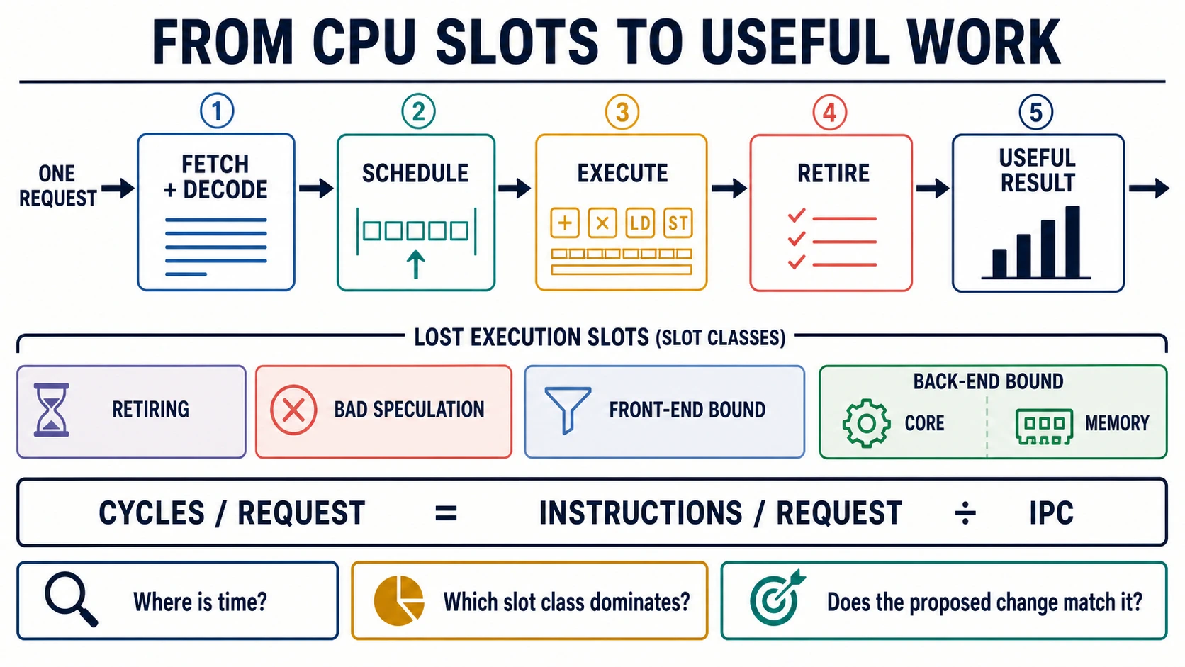
Modern cores fetch and decode instructions, place operations into scheduling structures, execute ready work, and retire results in architectural order. Out-of-order execution lets independent later operations run while an earlier operation waits. Superscalar execution lets more than one operation use different resources in a cycle. Neither escapes true dependency chains: if operation B needs A’s result, B waits.
Speculation predicts control flow so the pipeline can keep moving. A correct prediction hides decision latency. A wrong prediction discards speculative work and refills the useful path. This is why branch count alone is weak evidence; prediction accuracy, recovery cost, and the work behind each branch matter.
Four places execution slots go
A top-down analysis asks how potential pipeline slots were used. On supported Intel tooling, the first-level families are commonly expressed as retiring, bad speculation, front-end bound, and back-end bound. Treat them as questions:
- Retiring: useful operations reached retirement. A high value can mean productive work, but it can also expose an instruction-heavy algorithm doing avoidable work.
- Bad speculation: slots were consumed by work that could not retire, often after a mispredicted path or machine clear.
- Front-end bound: the core could not supply usable operations quickly enough because of fetch, decode, instruction-cache, translation, or instruction-footprint limits.
- Back-end bound: operations were available but could not execute because required execution resources or data were unavailable. The next split is often core-resource pressure versus memory-related waiting.
The categories prevent counter folklore. A branch rewrite matches bad speculation; a smaller instruction footprint may match a front-end limit; a layout change may match memory-bound back-end time; vectorization may match suitable compute-bound work. Applying one of those changes to the wrong class can reduce instructions and still increase cycles.
The labels are not portable facts. Processor models expose different events, virtual machines may restrict or virtualize counters, event multiplexing can scale estimates, and simultaneous hardware threads change attribution. Record the CPU model, firmware, kernel, tool, event encoding, privilege boundary, affinity, run state, and whether counters were multiplexed.
The arithmetic that connects counters to requests
Use cycles per operation or cycles per request for a fixed useful-work boundary:
cycles/request = instructions/request ÷ instructions/cycle
CPU service time/request ≈ cycles/request ÷ effective cycles/second
IPC is a ratio, not an objective. Increasing IPC while doing twice as many instructions can lose. Decreasing IPC while eliminating most work can win. Normalize both numerator and denominator to the same completed, correct population; otherwise rejected requests, retries, or changed outputs contaminate the comparison.
Decompose request demand before debating a function:
cycles per correct request
├── application user cycles
│   ├── parse and validate
│   ├── policy and ranking
│   └── encode response
├── runtime and allocator cycles
├── kernel and protocol cycles
├── repeated or abandoned work
└── background work charged to foreground capacity
Sampling profiles answer where on-CPU samples appear. Counters help answer why the core did not retire more useful work. Wall-clock traces answer whether CPU demand is actually on the user-visible critical path. The three must agree before a low-level change earns priority.
Reading the modeled counter packet
The Mercury fixture compares equal request outputs on one homogeneous pinned core set:
| Measure | Baseline | Candidate | Interpretation |
|---|---|---|---|
| instructions/request | 3,200 | 2,800 | candidate executes 12.5% fewer |
| IPC | 2.0 | 1.4 | candidate makes less retirement progress per cycle |
| cycles/request | 1,600 | 2,000 | CPU demand rises 25% |
| retiring slots | 50% | 35% | a smaller share becomes retired work |
| back-end bound | 35% | 50% | candidate waits more in the back end |
| candidate back-end split | — | 8% core, 42% memory | investigate data supply before arithmetic |
Suppose the profile also moves from a compact table scan to pointer-following nodes. The causal hypothesis is not “IPC is bad.” It is: the new representation saves instructions but destroys locality; dependent loads expose memory latency, reduce available independent work, and increase cycles per lookup. Test that by restoring layout while holding algorithm and output constant, measuring relevant cache/TLB events supported by this CPU, and checking whether cycles and the memory-bound share move together.
Counter names do not prove the story alone. A cache-miss count needs an access population and penalty context. A stall event may overlap another event. Prefetch can create traffic that never appears as demand-load misses. Start with a broad slot classification, then refine only the dominant class with model-specific guidance.
A profile-to-counter decision tree
Is CPU service demand material to the objective or capacity limit?
├── no  → fix the dominant wait, queue, dependency, or architecture first
└── yes → is the hot path tied to the same completed useful work?
    ├── no  → repair attribution and normalization
    └── yes → which top-level slot class dominates or regressed?
        ├── bad speculation → inspect branch outcomes and recovery
        ├── front end       → inspect instruction footprint, fetch, decode, iTLB
        ├── back end/core   → inspect ports, dependencies, divider, contention
        ├── back end/memory → inspect layout, locality, cache/TLB, NUMA
        └── retiring        → reduce necessary instructions or change algorithm
“Dominates” needs a comparison: against the baseline, a matched cohort, or a credible architecture-specific bound. A percentage can rise because another category shrank. Preserve absolute cycles per useful operation beside shares.
Vector work: ceiling before implementation
Vector instructions apply one operation to multiple lanes, but vector width is not speedup. Data must be eligible, laid out for efficient access, and processed with enough lane occupancy. Remainders, gathers, conversions, dependencies, and frequency behavior can reduce the gain.
For the teaching fixture, 52% of CPU work is vectorizable, an eight-lane implementation reaches 68% lane efficiency, and CPU demand is 62% of end-to-end time. The vectorized component’s idealized speedup is 8 × 0.68 = 5.44. Amdahl’s law bounds CPU speedup:
CPU ceiling = 1 / ((1 - 0.52) + 0.52 / 5.44) ≈ 1.737×
End-to-end speedup is smaller:
request ceiling = 1 / ((1 - 0.62) + 0.62 / 1.737) ≈ 1.357×
That ceiling assumes the change adds no setup, bandwidth, contention, thermal, or correctness cost. If a 1.36× theoretical request ceiling cannot justify complexity and portability cost, stop before writing intrinsics. If it can, measure lane occupancy, cycles per correct item, sustained frequency, memory traffic, and whole-request latency.
Topology changes the experiment
CPU affinity is an experimental boundary. Migration can mix counter populations, disturb caches, and move work across NUMA locality. Pinning can improve repeatability while creating an unrealistic production placement. Record both: use a pinned diagnostic experiment to isolate a mechanism, then validate the deployment scheduler and placement policy.
On simultaneous multithreading, two logical CPUs share core resources. A throughput win may coincide with worse single-request latency. Across sockets, data can be physically closer to one core than another. Interrupts and kernel work can consume cycles outside the application thread. Chapter 10 develops memory and NUMA mechanisms; here the operational rule is to identify the core, hardware-thread sibling, socket, and memory placement before interpreting small differences.
Turbo is a state, not a specification
A short isolated benchmark may run at a higher frequency than a sustained all-core workload. Thermal saturation, package power, cooling, vector instruction mix, and neighboring activity can change effective frequency. Therefore report elapsed time, cycles, and the platform’s supported frequency or residency evidence when available. Warm the system to the state the claim describes.
Use at least these states:
| State | What it tests | Common invalid transfer |
|---|---|---|
| isolated, pinned | mechanism and repeatability | claiming fleet capacity |
| sustained nominal | steady service demand and frequency | ignoring overload |
| full-core load | package power and shared resources | treating it as single-tenant latency |
| colocated/noisy | scheduler and contention exposure | blaming the code without placement evidence |
| recovery/replay | background amplification | extrapolating from normal traffic mix |
If the proposed optimization wins only in the cold first seconds or on one core topology, say so. A deployment needs a workload and platform envelope, not the best run.
When the architecture wins
Micro-optimization matters when CPU service demand materially limits throughput, cost, energy, or latency; the hot work belongs to correct outputs; a measured stall class matches the change; and the gain survives sustained production states. It does not matter merely because a loop looks inefficient.
Changing an O(n) lookup to a bounded indexed lookup, eliminating duplicate parsing, cancelling abandoned work, or removing retry amplification can erase more instructions than tuning a leaf function. Conversely, a stable 8% cycles-per-request reduction across billions of homogeneous operations may justify specialized code. Scale and repeatability decide—not aesthetic preference.
Field card: a defensible CPU claim
Before accepting a CPU optimization, record:
- Useful-work boundary: completed correct requests, records, bytes, or another invariant output.
- System consequence: objective, capacity, cost, or energy currently constrained by CPU demand.
- Experiment envelope: workload, input distribution, binary/compiler, CPU, topology, affinity, kernel/tool, temperature state.
- Where: matched on-CPU profile and attribution.
- Why: broad counter classification, then model-specific events for the dominant class.
- Arithmetic: instructions, cycles, IPC, elapsed time, and demand per useful operation.
- Alternatives: algorithm, layout, batching, cancellation, or architecture change.
- Validity: repeated trials, correctness check, sustained state, uncertainty, and transfer limit.
Applied exercise
Run the file-backed model with node examples/performance-engineering-system-design-handbook/part-02/cpu-execution/verify.mjs. Explain why “12.5% fewer instructions” loses, identify the next experiment from the slot split, then recalculate the vector ceiling if CPU represents only 35% of end-to-end time. Finally, write one sentence that would falsify your preferred optimization.
The decision is conditional: use CPU-level optimization only after proving CPU service demand is a material system constraint and the measured stall class matches the proposed change. The next layer is data supply—cache, locality, translation, and NUMA—which explains many back-end stalls that source code alone cannot.
Sources and evidence scope
- Intel VTune Profiler 2025.4, Top-down Microarchitecture Analysis supplies the processor-specific slot methodology. Its event mappings and thresholds do not transfer automatically across CPU models.
- Linux kernel workload tracing documentation describes
perfas an interface over hardware and software events; perf security documentation bounds access and data-exposure claims. - Linux arm64 perf documentation documents counter-width, guest/host, and heterogeneous-core caveats. Those details are architecture-specific but demonstrate why counter provenance matters.
- The Mercury numbers, slot shares, and vector ceilings are modeled teaching evidence in
examples/performance-engineering-system-design-handbook/part-02/cpu-execution/; they are not hardware measurements.