Performance Engineering and System Design Handbook / Chapter 7
Bottlenecks, Constraints, and Causal Diagnosis
Locate the constraint that limits user-visible goodput, distinguish cause from symptom, and choose discriminating tests before optimizing.
Preparing audio…
Audio edition
Bottlenecks, Constraints, and Causal Diagnosis
At 10:17 UTC, Mercury API’s interactive-search p99 rose from 230 ms to 690 ms. Offered load held at 1,200 requests/s, but correct goodput fell from 1,120 to 920 responses/s. The first incident message blamed the database because its connection pool showed 96 of 96 connections active.
The rest of the packet resisted that conclusion:
| Signal | Baseline | Regression |
|---|---|---|
| database-pool wait p99 | 8 ms | 310 ms |
| database-query service p99 | 42 ms | 44 ms |
| enrichment dependency p99 | 55 ms | 250 ms |
| database-connection hold p99 | 38 ms | 275 ms |
| active database connections | 72 | 96 of 96 |
The database pool was saturated, but query execution had barely changed. Joined traces showed the new enrichment call occurring while the application still held a connection. The pool was the waiting location. The remote call extended resource ownership. The release regression was the change that made it possible. “Database bottleneck” collapsed four different facts into one label.
The diagnostic method is to preserve those distinctions until a test can eliminate alternatives. Optimize the current system constraint or the dominant term in the user-visible critical path; otherwise require explicit strategic justification.
Name the thing before trying to remove it
A hot spot has concentrated activity: a busy function, shard, lock, core, tenant, or route. It may have spare capacity or sit off the critical path.
A symptom is an observed departure from an objective: higher latency, lower goodput, growing age, errors, excess CPU per result, or missed freshness. Symptoms define the investigation but do not explain themselves.
A bottleneck is the resource or mechanism currently limiting additional useful system output in the stated workload and state. Its identity can change with request mix, skew, failure, recovery, or an optimization.
A constraint is broader: any bound that limits the goal. It may be physical capacity, serialization, a dependency objective, correctness, a quota, cost, deployment risk, or an organizational change rate.
A root cause is the condition or change whose removal, under the relevant causal model, prevents or materially reduces the symptom. One incident can have several contributing causes and one current bottleneck. Removing the trigger may expose an older capacity weakness; increasing capacity may mask the trigger without correcting ownership.
Use names with boundaries: “the 96-slot application database pool limits correct interactive-search goodput during enriched traffic because connections are held across a remote dependency.” That claim can be tested. “The database is slow” cannot.
Account for work before accounting for utilization
Conservation-of-work reasoning asks where offered work goes and what resources each outcome consumes. Over an interval, attempts become admitted work, rejections, completions, cancellations, timeouts, and retained backlog. Useful completions are only one branch. Retries, abandoned queries, duplicate serialization, failed speculation, lock spinning, and recovery traffic consume capacity without adding correct goodput.
For resource r, a simple demand model is:
resource work per second = Σ (class arrival rate × demand per class on r)
Demand must use the resource’s unit: CPU-seconds/request, connection-seconds/request, bytes/request, I/O operations/request, or lock-hold-seconds/request. Divide available resource service per second by demand per correct result to estimate a scoped upper bound. Reconcile against observed goodput; a large gap is a clue about waiting, waste, skew, or a wrong boundary.
Mercury’s illustrative class demands are:
| Request class | Mix | CPU demand | Database-connection hold | Storage operations |
|---|---|---|---|---|
| basic search | 72% | 5 ms | 9 ms | 1 |
| enriched search | 28% | 7 ms | 72 ms | 1 |
The weighted CPU demand is 0.72 × 5 + 0.28 × 7 = 5.56 ms/request. Weighted connection demand is 0.72 × 9 + 0.28 × 72 = 26.64 ms/request. The connection figure is a mixture average, not evidence that each request holds a connection for 26.64 ms. At 1,200 requests/s it implies roughly 32 connection-seconds/s of offered ownership under the assumed mix, before retries. The 96-slot pool should not saturate from that average alone; the observed 275 ms enriched hold tail, correlated arrivals, waiting transactions, or repeated work must be reconciled.
This is why work-normalized metrics complement utilization. CPU percent can rise because goodput rises, because waste rises, or because completions fall while retries grow. CPU-seconds per correct result separates those stories. Bytes per durable write, I/O per accepted event, lock-hold time per successful mutation, and dependency attempts per terminal user outcome expose amplification.
Five mechanisms produce similar latency lines
The same end-to-end symptom can come from different mechanisms:
- saturation: offered demand reaches effective service capacity, so work queues;
- contention: actors compete for a shared resource and spend time waiting, spinning, retrying, or invalidating one another;
- serialization: an ordering or ownership rule permits only one relevant action at a time;
- dependency wait: progress is blocked on another component, network exchange, quorum, or external state;
- coordination delay: useful work completes locally but the result waits for barriers, joins, consensus, stragglers, or scheduler decisions.
Each mechanism predicts different companion evidence. CPU saturation should show runnable work or scheduler delay at the relevant core or quota, not merely fleet-average CPU. Lock contention should show waiters and hold-time lineage. Dependency wait should appear in joined client spans and outcome rates. Coordination delay should leave idle or completed participants waiting for a laggard or condition.
The counterexample is the busiest-component rule. A telemetry encoder can consume the most CPU while an eight-slot storage semaphore limits completions. Making encoding twice as fast reduces local CPU but does not increase goodput because storage admits no more work. It may even worsen the system by delivering bursts to the semaphore faster and increasing queue variance. The changed variable is not whether encoding became cheaper; it is whether encoding was on the dominant critical path or constrained the completion rate.
Draw the critical path from joined events
The user-visible critical path is the longest dependency-respecting chain that determines a particular completion. It is not necessarily the component with the largest aggregate time or resource use. Parallel work off that chain may be expensive and economically worth optimizing, but reducing it will not shorten that request unless it changes contention, scheduling, or a future path.
For a search request, join admission, queue, CPU execution, connection acquisition, query, enrichment, serialization, and response events by request and attempt. Mark ownership intervals separately from active service. In the regression trace:
checkout DB connection
  query: 44 ms
  enrichment RPC: 250 ms
release DB connection
The remote call is on the response critical path and inside the connection-ownership interval. Pool wait on later requests is a downstream consequence. Summing dashboard p99 values would not prove this ordering; one joined trace population plus distribution-level confirmation can.
Critical paths vary by class and outcome. A cache hit, cache miss, timeout, retry success, and partial result may follow different graphs. The p99 path can also switch after an optimization. Preserve request class, version, tenant, region, failure domain, and terminal outcome in the evidence.
Off-critical work still matters when it competes for a critical resource. An asynchronous audit task may not delay its parent directly, yet its I/O can saturate the device needed by foreground queries. Causal analysis must include resource-interference edges as well as control dependencies.
USE, RED, and normalized work answer different questions
Three lenses reduce blind spots when they remain distinct.
The USE method asks, for every resource, about utilization, saturation, and errors. Resource means a physical or meaningful software resource such as CPU, memory capacity, device I/O, a thread pool, or a connection pool. Utilization describes busy time or degree used; saturation describes extra work the resource cannot service, often queued. It is a systematic early search for resource constraints.
The RED method asks, for every service, about request rate, error rate, and duration distributions. It keeps the user-facing service behavior visible while resources are inspected. Rate without offered/admitted distinction can still mislead, and “duration” needs the population discipline from Chapter 5.
The work-normalized view asks how much resource and amplification each correct unit consumes. It connects service symptoms to mechanism and economics.
| Question | Strong first lens | Necessary companion |
|---|---|---|
| Which machine resource is under pressure? | USE | class demand and user effect |
| Which service boundary is failing its objective? | RED | offered/admitted/correct outcome scope |
| Did a change make each result more expensive? | work-normalized | resource saturation and critical path |
| Is a low-utilization resource still delaying work? | saturation/wait evidence | interval, quota, partition, and ownership |
None is a root-cause oracle. USE can locate a saturated pool but not explain why ownership grew. RED can identify a service regression but not distinguish queue wait from service. Normalized cost can show amplification while hiding a rare critical-path stall. Start broad, then form a mechanism-specific causal claim.
Linux Pressure Stall Information can quantify CPU, memory, and I/O stall time, including short pressure intervals obscured by long averages. It is a useful saturation signal in supported Linux environments. It does not identify the code, request class, or upstream change that caused pressure. A zero host-level PSI signal also does not rule out a lock, pool, partition, remote dependency, or cgroup limit outside the observed boundary.
Turn correlation into a discriminating test
A causal graph makes assumptions visible. For the Mercury regression, a compact graph is:
release R17
   └─ holds DB connection across enrichment
          ├─ longer connection ownership
          │      └─ pool saturation ──> pool wait ──> response latency
          └─ remote slowdown ─────────> response latency
Competing explanations include slower database execution and host CPU saturation. Each hypothesis must predict observations that could distinguish it:
| Hypothesis | Expected if true | Evidence already against it | Cheapest next test |
|---|---|---|---|
| database execution slowed | query service and database demand rise | query p99 changed only 42→44 ms | compare query spans/plans for matched class |
| connection held across enrichment | hold overlaps RPC; pool wait follows long holds | none in packet | join checkout/release and RPC spans; disable enrichment for a controlled cohort |
| host CPU saturated | run queue or quota stall aligns with delay | host average modest; wait dominated by pool | inspect per-core/quota saturation and off-CPU wait |
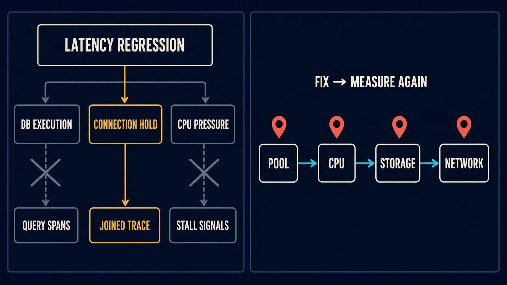
The least expensive decisive test is not necessarily the cheapest measurement. A metric already on a dashboard costs almost nothing but may leave all hypotheses alive. Joined connection-ownership and enrichment spans directly test temporal overlap. A small controlled cohort that performs enrichment after releasing the connection tests intervention, provided request mix, correctness, and downstream load remain comparable.
Use four questions for every proposed test:
- What observation differs between the leading hypotheses?
- Can the measurement preserve request class, outcome, and time ordering?
- Could the test itself change load, cache state, scheduling, or failure behavior?
- What result would reverse the proposed decision?
If no result could reverse the decision, the activity is confirmation theater, not diagnosis.
A causal diagnosis worksheet
Record one row per claim rather than one row per dashboard:
| Field | Mercury entry |
|---|---|
| symptom and objective | interactive-search p99 690 ms vs 250 ms target; correct goodput 920/s |
| boundary and state | gateway admission to correct terminal response, release R17, normal dependency state except enrichment latency |
| change | connection release moved after enrichment call |
| proposed mechanism | longer ownership saturates 96-slot pool and queues later requests |
| alternatives | database execution; CPU quota; request-mix shift; retry amplification |
| predicted signatures | hold overlaps RPC; stable query service; pool wait follows long enriched holds |
| discriminating test | joined spans plus matched enrichment-disabled cohort |
| correctness guard | same result fields and database transaction boundary |
| transfer limit | applies to this release, traffic mix, pool, and dependency state |
| decision threshold | restore hold distribution and goodput without shifting errors or stale results |
The worksheet prevents a profiler screenshot or correlated metric from becoming the conclusion. It also records what the intervention must not break.
Differential profiles attribute changed resource use
A conventional profile shows where sampled resource time accumulated in one run. A differential profile compares matched baseline and candidate populations to show where stack contribution increased or decreased. CPU flame graphs are one form; off-CPU profiles, allocation profiles, lock traces, I/O attribution, and query plans answer other mechanisms.
Match workload, duration, warm-up, version, sampling frequency, symbolization, and operating state. Normalize appropriately—per unit time for capacity, per correct request for efficiency, or per class when mix changed. A larger frame can reflect more offered work rather than higher demand per request. A vanished frame can mean inlining, symbol failure, sampling error, or work moved to a different process.
Differential profiling is most valuable after the causal question is stated: “Which stacks account for the extra 1.8 CPU-ms per correct enriched response?” It is weaker as an unguided hunt for the reddest frame. Brendan Gregg’s USENIX flame-graph work documents differential and off-CPU variants; the visualization does not supply experimental control or prove that a changed stack caused the user symptom.
Before/after attribution also needs a counterfactual. Alternate versions under comparable load, randomize cohorts, use a controlled replay, or exploit a clear rollback where feasible. Time-series coincidence with a deployment is strong change evidence but can be confounded by traffic, cache, dependency, autoscaling, and recovery changes.
Expect the bottleneck to migrate
Once Mercury releases connections before enrichment, connection-pool wait collapses and correct goodput rises. The old bottleneck claim expires. The fixture models a sequence of new constraints:
- after connection ownership is corrected, application CPU serialization limits modeled capacity near 1,760 requests/s;
- after serialization demand falls, storage IOPS limits it near 2,050 requests/s;
- after write coalescing, network egress limits it near 2,380 requests/s.
These capacities are illustrative decision points, not measured production results. Their purpose is to show that throughput improvements should be accompanied by a predicted next constraint. If the observed migration differs, the model omitted demand, coupling, or a failure mode.
Resource demand per class predicts migration more reliably than a ranked list of current utilization. A mix shift toward enriched searches increases connection and network demand faster than basic-search CPU demand. A regional failure may add cross-region bytes and coordination delay. Recovery may move the constraint to storage repair or cache fill. Re-run the bound for nominal, skewed, overloaded, failed, and recovering states.
A dangerous local “fix” is increasing the connection pool from 96 to 128. Acquisition latency may fall briefly, so the pool dashboard improves. If the database is already near its I/O or lock limit, extra concurrency can increase query service time, memory, and contention, reducing global goodput. The local metric improves while the system objective worsens. Test pool changes against end-to-end correct goodput, database demand per result, wait and service distributions, errors, and recovery behavior—not pool wait alone.
Stop when the next improvement does not pay
Optimization has opportunity cost and risk. Continue while the expected value of relieving the constraint exceeds engineering, infrastructure, operational, correctness, and migration cost under uncertainty.
A practical stopping record includes:
- current objective gap and population affected;
- evidence that the target is still the constraint or dominant critical-path term;
- modeled upper bound on user, capacity, or cost improvement;
- experiment and rollout cost;
- regression and correctness risk;
- lifetime of the benefit before growth or architecture change;
- the next measurement that would materially alter expected value.
Amdahl-style upper bounds from Chapter 4 remain useful. If a function is 3% of end-to-end latency and does not constrain throughput, eliminating it cannot justify a quarter of migration risk merely because it is easy to profile. Strategic work can still be valid: reducing an off-path cost may enable a future feature, retire a platform, or create safety margin. Name that strategic objective instead of calling it the current bottleneck.
Stop an incident investigation when the objective is restored, causal evidence is sufficient for the operational decision, and remaining uncertainty has an owner and bounded risk. Stop a performance program when marginal benefit falls below the agreed economic or reliability threshold—not when every component is equally utilized. Balanced utilization is neither achievable nor desirable in many architectures.
Work the telemetry packet
Using only the Mercury packet and fixture:
- Define the symptom population and terminal success.
- Rank the four hypotheses: connection held across enrichment, slower query execution, host CPU saturation, and request-mix shift.
- Write one predicted observation that would support and one that would weaken each.
- Choose the least expensive discriminating test, including a correctness guard.
- Explain why increasing the pool can improve acquisition wait while worsening global goodput.
- After the ownership fix, identify the metrics needed to validate the modeled migration to CPU, storage, and network constraints.
The fixture ranks the declared hypotheses by support minus contradictions only to verify that the evidence packet is internally coherent. That scoring rule is not a general causal algorithm. Human review must challenge omitted causes, dependence, measurement error, and intervention risk.
$ node examples/performance-engineering-system-design-handbook/part-01/queues-and-causality/verify.mjs
queues: verified low=3/7/12/27/57 ms high=18/42/72/162/342 ms, burst excess=280, bound=180
causality: ranked=connection held across enrichment, weighted CPU=5.56 ms, connection=26.64 ms
Decision rules
- Define symptom, boundary, workload, state, objective, and correct outcome before naming a bottleneck.
- Distinguish hot spot, waiting location, limiting constraint, trigger, contributing condition, and root cause.
- Reconcile offered work into correct goodput, failures, retries, cancellations, and backlog; normalize resource use per correct result.
- Trace user-visible critical paths with joined events and include resource-interference edges from off-path work.
- Use USE for resource search, RED for service behavior, and work-normalized demand for mechanism and economics; none proves causality alone.
- Rank competing hypotheses by predicted evidence and choose a test capable of reversing the decision.
- Match differential profiles by workload, class, state, and normalization; do not optimize the largest frame by appearance.
- Predict and then measure bottleneck migration after every material change.
- Reject local improvements that reduce a component metric while harming correct end-to-end goodput, tails, cost, or recovery.
- Stop when the scoped objective is met or the next bounded improvement no longer justifies its full risk-adjusted cost.
You can now describe demand, objectives, units, populations, queues, and causal constraints without collapsing them into one dashboard. The design loop assembles those pieces into a repeatable practice: estimate, draw, budget, choose overload behavior, specify evidence, and record what would force redesign.
Sources and evidence scope
- Brendan Gregg, “The USE Method” defines the utilization, saturation, and errors resource checklist and discusses software resources such as locks and thread pools. It is an investigation strategy, not proof that the first saturated resource is the root cause.
- Grafana Labs, “The RED Method: How to Instrument Your Services” records Tom Wilkie’s rate, errors, and duration service lens. The source does not replace population definitions, offered/admitted accounting, or causal tests.
- Linux kernel Pressure Stall Information documentation defines CPU, memory, and I/O stall signals. PSI is environment-specific pressure evidence and cannot identify an application root cause by itself.
- Brendan Gregg, “Visualizing Performance with Flame Graphs,” USENIX ATC 2017 covers standard, differential, and off-CPU flame graphs. Profiles attribute sampled resource activity under their collection method; they do not establish user impact or causal transfer without a matched experiment.
- OpenTelemetry trace semantic conventions support consistent operation boundaries and attributes across signals. Convention status and versions vary; joined causal evidence still requires application ownership, class, attempt, and outcome semantics.
- The Mercury packet, demand table, hypothesis ranking, and migration capacities are modeled teaching fixtures. The verifier establishes arithmetic and internal consistency, not production causality or external validity.